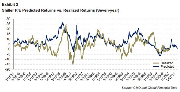
In this piece, I’m going to present and explain a simple, easy-to-understand method of forecasting stock market returns on the basis of valuation. I’m then going to insert the popular Shiller CAPE into the method to assess how well the historical predictions fit with the actual historical results. As you can see in the chart below, they fit almost perfectly, across 133 years of available data (no arbitrary exclusions). The correlation coefficient is a fantastic 0.92.
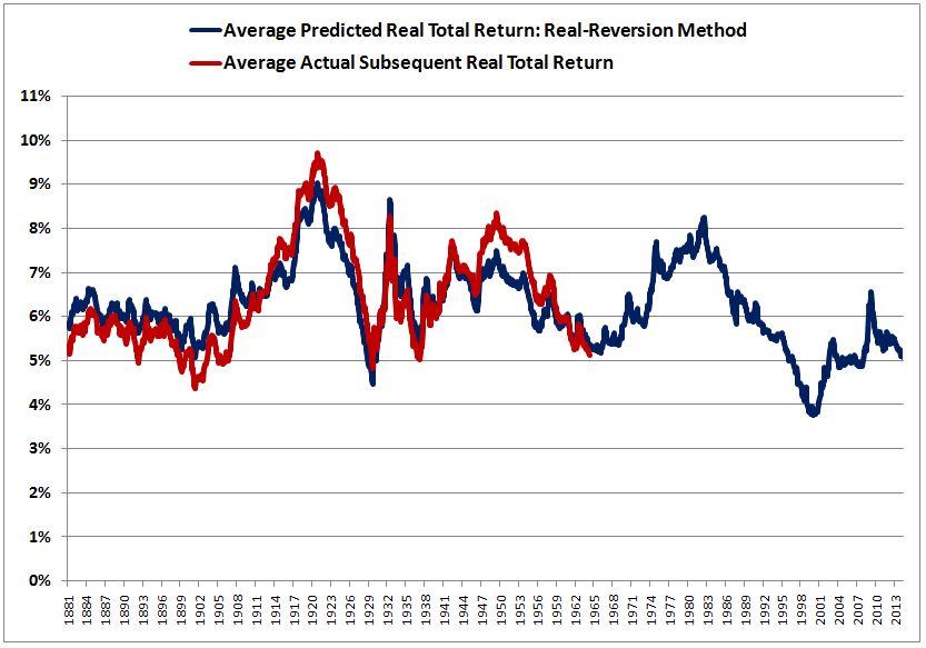
After presenting the chart, I’m going to demonstrate that its tight correlation is an illusion. I’m going to carefully flesh out its subtle trick, a trick that is ultimately hidden in every chart that purports to use valuation to accurately predict returns in historical data. Such a feat cannot be accomplished–the historical data will not allow it.
Now, let’s be honest. When we build charts in finance and put them on display, our primary motivation isn’t to “spread truth.” It’s to “talk our books”, broadcast to the world that the views and positions that we’re already emotionally and financially tied down to are right, and that those of our opponents and counterparties are wrong.
To that end, I might come up with a chart that really nails it. But so what? For all you know, the chart could have been the product of hours upon hours of searching, sifting, tweaking, and ultimately selectively discarding whatever didn’t fit with the thesis that I was trying to convey. Not knowing the process through which I arrived at the chart, how can you be confident that it represents an unbiased sampling of the possibilities? Why should you believe that its projections will hold true in the data that actually matter–the unsearched, unsifted, untweaked, undiscarded data of the future?
Ask yourself: is it possible that one carefully put-together chart out of a hundred might happen to fit well with a desired thesis, for reasons that are coincidental? If the answer is yes, then you can rest assured: that’s the chart that defenders of the thesis are going to end up showing you, every time. They’re going to search for it, find it, and put it on display–not because they know that it represents truth (they don’t), but because it persuasively communicates what they want to be true, and what they want you to believe is true.
The Drivers of Returns: Dividends and Per-Share Growth in Fundamentals
From January 1871 to today, U.S. equities have produced an average real total return of around 6% per year. We can conceptualize this return as coming from two different sources: (1) real growth in stable per-share fundamentals–book values, revenues, smoothed earnings (e.g., Robert Shiller’s 10 year average of EPS), etc.–and (2) real dividend payments that are reinvested into the equity markets and that compound at the equity rate of return.
The relative contribution of growth and dividends to real total return has changed over time, but the change hasn’t mattered much to the 6% number, because the two sources of return are fungible and inversely-related. For a given level of profit, a higher dividend payout means less reinvestment and less per-share growth. A lower dividend payout means more reinvestment and more per-share growth.
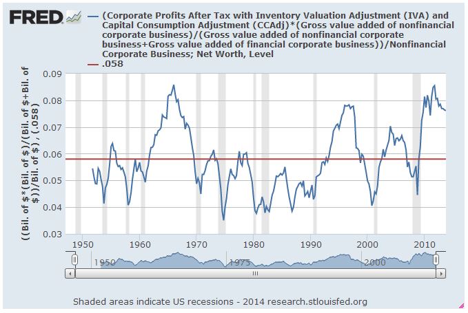
It is not a coincidence that U.S. equities have produced an average real total return of around 6% throughout history. That number matches the U.S. Corporate Sector’s average historical return on equity (ROE) of around 6%. The following chart shows the ROE for U.S. national corporations (non-financial) from 1951 to 2014 (FRED):
In theory, the average real total return that accrues to shareholders should match the average corporate ROE. For a simple proof, assume that the following premises hold true over the very long term:
(1) The corporate sector operates at a 6% average ROE (generates a 6% average profit on its true book value, defined to mean assets at replacement cost minus liabilities).
(2) Shares trade, on average, at “fair value”, which we will assume is equal to true book value.
It follows that either:
(1) the 6% average profit will be internally reinvested, and therefore added to the book value each year, with the result being 6% average growth in the book value, and therefore 6% average growth in the smoothed earnings, given that the corporate sector operates at a constant average ROE over the long-term, or
(2) the 6% average profit will be paid out as a dividend, in which case it will directly produce an average 6% return for shareholders (if shares trade, on average, at their book values, then a distributed dividend equal to 6% of the book value will also equal 6% of the market cap, therefore a 6% yield), or
(3) corporations will opt for some combination of (1) and (2), some combination of growth and dividends, in which case the sum will equal 6%.
The 6% will be a real 6% because inflation–i.e., changes in the price index–will change the nominal value of the assets that make up the book, properly accounted at replacement cost. By our assumption (1), changes in the price index will not drive changes in the average ROE (and why should they?), therefore they will pass through to the average smoothed earnings, preserving the 6% inflation-adjusted number underneath.
Now, we can loosely test this logic against the actual historical data. The following chart shows the trailing 70 year real return contribution from per-share growth (gold) and dividends reinvested at fair value (green) back to 1881, the beginning of the data set:
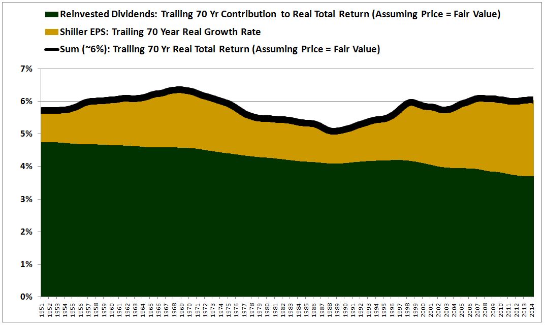
(Details: After presenting a non-trivial chart, I’m going to add a “details” section that rigorously describes how the chart was created, so that interested readers can reproduce its content for themselves. Uninterested readers should feel free to ignore these sections. In the above chart, we approximate the real return contribution from per-share growth using the real growth rate of Robert Shiller’s 10 year average of inflation-adjusted EPS, a cyclically-stable metric. We approximate the real return contribution from dividends reinvested at fair value by making two fake indices for the S&P 500: (1) a fake real total return index and (2) a fake real price return index. In these fake indices, we replace each historical market price with whatever price would have made the Shiller CAPE equal to exactly 15.3, its 133 year geometric average. To calculate the annual real return contribution from the reinvested dividend over a trailing period of X years, we take the difference between the annual returns of the two indices over the X year period. That difference is the reinvested dividend’s contribution to the real return on the assumption that shares always trade at “fair value.”)
As you can see in the chart, the logic checks very closely with the actual historical data, provided that we use a long time horizon. The average of the black line is 5.78%, roughly equal to the average corporate ROE of 5.80%. Notice that as the return contribution from growth (yellow) rises, the return contribution from dividends (green) falls, keeping the sum near 6%. This is not a coincidence. It doesn’t matter what relative share of profit the corporate sector chooses to devote to growth or dividends; over the long-term, the sum is conserved.
Formally, we can express the long-term average relationship between ROE, real total return to shareholders, real per-share growth in fundamentals, and the real return contribution from reinvested dividends, in the following equation:
ROE = Sustainable Real Total Return to Shareholders = Real Per-Share Growth in Fundamentals + Real Return Contribution From Reinvested Dividends = 6%
Now, to increase the return contribution from one source–say, growth–without reducing the return contribution from the other–dividends–the corporate sector can lever up. But this won’t refute the equation, because if the corporate sector levers up, it will increase its ROE, either by increasing its earnings at a constant book value (borrowing funds and investing in new assets that will provide new sources of profit), or by reducing its book value at a constant earnings (borrowing funds and paying them out as dividends–i.e., adding liabilities without adding assets). The assumption is that if the corporate sector tries to use leverage to boost its ROE above the norm, the leverage will have a stability cost that will show up in the future, during times of economic distress, pushing profitability down and ensuring that the average long-term ROE stays close to the norm.
In a similar manner, to increase the return contribution of one source while maintaining the return contribution of the other source constant, the corporate sector can try to raise funds by selling equity. But if, as we’ve assumed, shares trade on average at fair value, and the funds are deployed at an average ROE of 6%, then, whatever gets added–higher absolute growth, higher absolute dividends–will be added with a commensurate dilution that leaves the aggregate return contribution unchanged on a per-share basis.
Note that we haven’t mentioned share buybacks and acquisitions here because they have the same effect on a total return index as reinvested dividends. The corporate sector can take money and buy back its shares in the market, indirectly increasing the number of shares that remaining shareholders own, or it can pay the money out to shareholders as dividends, which they will reinvest, directly increasing the number of shares they own.
Now, in addition to growth and dividends, there’s one other crucial factor that impacts returns–changes in valuation. The assumption, of course, is that valuation reverts to the mean, and that any contributions that changes in it make to returns, whether positive or negative, will cancel out of the long-term average.
Suppose, for example, that a bubble emerges in the stock market, and that the valuation at time t rises dramatically above the mean. Whoever sells at t will enjoy a return that is significantly higher than the normal real value of 6%. But that return will be fully offset by the proportionately lower return that the buyer at t will have to endure, as the elevated valuation falls back down. Thus, if you average real returns across all time periods, the bubble won’t affect the 6% number. Nothing will affect that number except the sustainable drivers of real equity returns: fundamental per-share growth and reinvested dividends.
The tendency of valuation to mean-revert is precisely what allows us to use it to estimate long-term future returns. We know what long-term future returns are going to be, on average, if shares are purchased at fair value, and if no subsequent changes in valuation occur: roughly 6%, the normal combined return contribution of growth and dividends. Therefore, we know what long-term future returns are going to be, on average, if shares are not purchased at fair value, but eventually revert to that value–6% plus or minus the boost or drag that the mean-reversion will introduce.
The Real-Reversion Method: A Technique for Estimating Future Returns
Here’s a simple but useful method, which I’m going to call “Real-Reversion”, that allows us to make specific return predictions for specific future time horizons. For a specified time horizon, take the 6% real total return that U.S. equities have historically produced and adjust that return to reflect the increase or decrease that a mean-reversion in valuation, if it were to have occurred at the end of the time horizon, would produce. To get to a nominal return, add a separate inflation estimate to the result.
The equations:
Real Total Return = 1.06 * (Mean_Valuation/Present_Valuation) ^ (1/t) – 1
Nominal Total Return = Real Total Return + Inflation Estimate
Here, t is the time horizon in years. Mean_Valuation is the mean to which the valuation will have reverted at the end of the time horizon. Present_Valuation is the present valuation.
On this equation, if the valuation is precisely at the mean, the predicted future return will be 6% per year. If the valuation is above the mean, the predicted future return will be 6% discounted by the annual drag that that the mean-reversion will produce over the time period. If the valuation is below the mean, the predicted future return will be 6% accreted by the boost that the mean-reversion will produce over the time period.
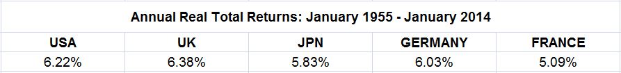
Of note, if we look at the historical real returns of other developed capitalist economies, we see that numbers close to 6% frequently come up. The following table shows the average annual real total returns for the US, UK, Japan, Germany and France back to 1955, a time when valuations were very close to the historical average (Shiller CAPE ~ 16 for the USA):
Notice that the “Real-Reversion” method uses valuation to estimate real returns, not nominal returns. Nominal returns have to be estimated separately, using a separate estimate of inflation over the time period in question. The reason the method has to be constructed in this way is that inflation hasn’t followed a reliable trend over the long-term, and doesn’t need to follow any trend. Unlike real equity returns, it isn’t driven by a factor, ROE, that mean-reverts. It’s driven by policy, demographics, culture, and supply dynamics–factors that can conceivably go in whatever direction they want to. If we try to incorporate it directly in the forecasting method, we will introduce significant historical error into the analysis.
Now, let’s plug the familiar Shiller CAPE into the method to generate a 10 year total return prediction for the present S&P 500. With the S&P 500 at 1940, the GAAP Shiller CAPE is approximately 26.5. If, over the next 10 years, we assume that it’s likely to revert to its post-war (geometric) mean of 17, we would estimate the future annual real total return to be:
1.06 * (17/26.5)^(1/10) – 1 = 1.4%
If we wanted a nominal number, we would add in an inflation estimate: say, 2%, the Fed’s present target. The result would be a 3.4% nominal annual total return. Note that we haven’t made any adjustments for the effects that emergent changes in dividend payout ratios and accounting practices (related to FAS 142 and also to the provable fact that corporations lied more about their earnings in the past than they do today) have had on the Shiller CAPE. To be fair, we also haven’t made any of the punitive profit-margin adjustments that valuation bears would have us make.
To give credit where credit is due, “Real-Reversion” is (basically) the same method that James Montier used in a recent piece on the Shiller CAPE. It’s a simplification of GMO’s general asset class forecast method–take the normal expected real return, and adjust it for the effects of mean-reversion. There really isn’t any other way to reliably use valuation to estimate long-term future equity returns–GMO’s method is essentially it.
In James’ piece, he showed the performance of the method across GMO’s preferred 7 year mean-reversion time horizon.
He explained:
“We simply revert the P/E towards average over the course of the next seven years and then add a constant to reflect growth and income (let’s call it 6% for simplicity’s sake). It does a pretty reasonable job of capturing realised returns. If anything, it tends to overpredict returns, rather than underpredict them (which is another of the charges levelled by the critics).”
The following is my recreation of the 7 year chart using Robert Shiller’s data:
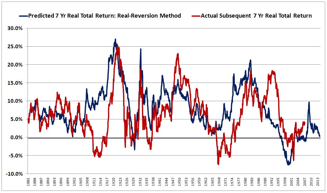
I would disagree that the method does a pretty reasonable job of capturing realized returns. In my view, it does a terrible job. The fit is a mess, with a linear correlation coefficient of only 0.51. That’s an awful number, particularly given that the expressions being correlated–“present valuation” and “future returns”–share a common oscillating term, present price. Analytically, those terms already start out with a trivial correlation between them (which is the reason the squiggles in the two lines tend to move in unison).
I would also disagree that the method tends to overpredict returns. It only tends to overpredict returns in the pre-war period. In the post-war period, it tends to underpredict them. The following table shows the frequency of 7 year underprediction, using a generous 17 as the mean (if we used the actual 133 year geometric average of 15.3, the underprediction would be even more frequent):
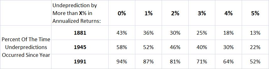
Since 1945, the method has underpredicted returns roughly 58% of the time. Since 1991, it’s underpredicted them roughly 95% of the time–half of the time by more than 5% annually. Compounded over a 7 year time horizon, that’s a big miss.
The fact that the method has failed to make accurate predictions in recent decades shouldn’t come as a surprise to anyone. Since early 1991, roughly the end of the first Gulf War, the Shiller CAPE has only spent 10 months below its assumed mean–out of a total of 278 months. There is no way that a forecasting method that bets on the mean-reversion of a valuation metric can produce accurate forecasts when the metric only spends 3.6% of the time at or below its assumed mean.
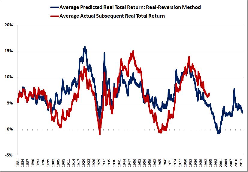
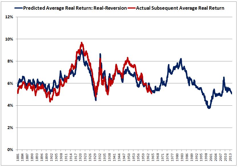
I prefer to look at return estimates over a 10 year period, because 10 years sets up a convenient comparison between the expected return for equities and the yield on the 10 year treasury bond. The following chart shows the performance of the method over a 10 year horizon, from 1881 to 2014:
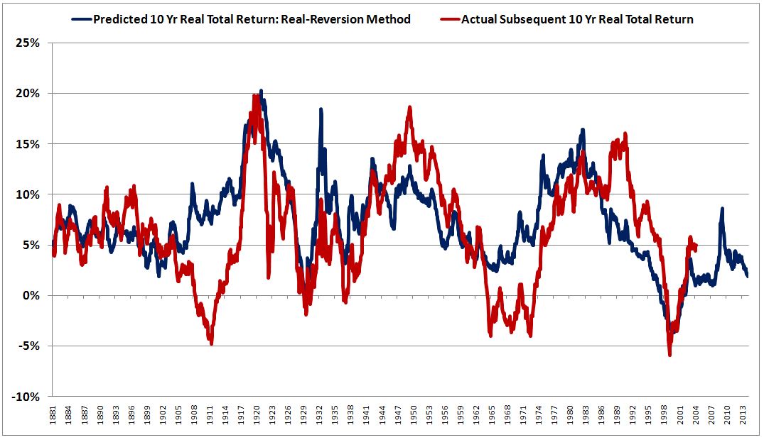
The correlation coefficient rises to 0.59–better, but still grossly inadequate.
Point-to-Point Comparison: “Shillerizing” the Returns
What we’re doing in the above chart is we’re comparing the predictions of the method at each point in time to the total returns that subsequently occurred from that point to a point 10 years out into the future. So, for example, we’re looking at the Shiller CAPE in February of 1991 at 17.3, we’re estimating a 10 year real total return of 5.8% per year (6% reduced by the drag of a 10 year mean reversion from 17.3 to 17), and then we’re comparing this estimate to the actual annual return that occurred from February of 1991 to February of 2001.
The problem, of course, is that from February of 1991 to February of 2001, the Shiller CAPE didn’t revert from 17.3 back down to the mean of 17, as the model assumed it would. Rather, it skyrocketed from 17.3 to 35.8. The actual real total return ended up being 13.5%, more than twice the model’s errant 5.8% prediction.
Ultimately, if the 6% normal return assumption holds true, then any time the Shiller CAPE ends a period with a value that is not 17, this same error is going to occur. We will have estimated the future return on the basis of a mean-reversion that didn’t actually happen; the estimate will therefore be wrong. So unless we expect the Shiller CAPE to always equal something close to 17, for all of history, we shouldn’t expect the model’s predictions to fit well with the actual historical results on a point-to-point basis. Point-to-point success in historical data is a highly unreasonable standard to impose on the method.
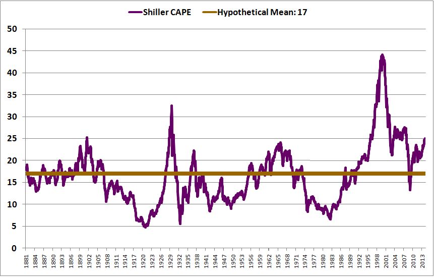
As you can see in the chart above, the Shiller CAPE has historically exhibited a very large standard deviation–equal to more than 40% of its historical mean–with extremes as low as 5 (early 1920s) and as high as 40 (late 1990s). 30% of the overall data set consists of periods in which it was below 10 or above 22. In those periods, the model should be expected to produce very incorrect results.
Indeed, if the model doesn’t produce incorrect results in those periods, then either the 6% normal real return assumption is wrong, or the two errors–the error in the 6% normal real return assumption and the error in the 10 year mean-reversion assumption–are by luck cancelling each other out. In other words, we’ve data-mined a curve-fit, a superficial exploitation of coincidental patterning in the data set. Obviously, if our goal is to build a robust model that will allow us to successfully predict returns out of sample, in the unknown data of the future, we shouldn’t want it to pass a backtest in such a spurious manner.
To get around the problem, we need to rethink what we’re trying to say when we issue future return estimates. We’re not trying to say that the future return will necessarily be what we predict–that would be hubris. Rather, we’re trying to make a conditional statement, that the return will be what we predict if our assumptions about 6% “normal” returns and mean-reversion in valuation hold true for the period. We’re additionally asserting that those assumptions probably will hold true–not always, but on average.
A better way to test the reliability of the method, then, is to test it on averages of points, rather than on individual points. To illustrate, suppose that we do the following: for each point in time, we use the method to generate an estimate of the future 10 year return, the future 11 year return, the future 12 year return, and so on, covering a 10 year span, all the way to the future 19 year return. We then calculate the average of each of these 10 estimates. We compare that average to the average of the actual subsequent returns over the same 10 year span: the actual subsequent 10 year return, the actual subsequent 11 year return, the actual subsequent 12 year return, and so on, all the way up to the actual subsequent 19 year return.
If, at a given point in time, the Shiller CAPE looking 10 years out just so happens to be abnormally high or low, our estimate of the future 10 year return will end up being incorrect. But, to the extent that the abnormality is infrequent and bidirectional, the error will get diluted and canceled by the other terms in the average. Assuming that deviations in the terminal Shiller CAPEs in the other years average out to the mean–which they generally should if we’re making reliable assumptions about mean-reversion–the averages of the predictions will still closely match the averages of the actual results.
This approach is similar to the approach that Robert Shiller famously uses to analyze earnings. When calculating earnings growth, he calculates the growth in the trailing 10 year average of earnings, not the growth in point-to-point earnings, which is highly cyclical. We’re doing the same thing with returns, which, on a point to point basis, are also highly cyclical. In a word, we’re “Shillerizing” them.
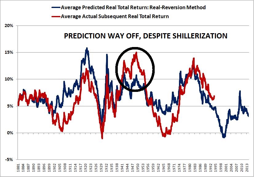
The following chart shows predicted and actual 10 year “Shillerized” returns from 1881, the beginning of the data set, to present:
(Details: For each point in the chart, the average of the return predictions 10, 11, 12, 13, 14, 15, 16, 17, 18, and 19 years out is compared to the average of the actual realized returns 10, 11, 12, 13, 14, 15, 16, 17, 18, and 19 years out.)
The correlation between the predicted returns and the actual returns rises to 0.72. Better, and certainly more visually pleasing, but still not adequate. To improve the forecasting, we need to take a closer look at the sources of error in the method.
Three Sources of Error: Why A Very Long Horizon is Needed
There are three sources of error in the method. These errors are:
(1) Growth Error: errors driven by historical variabilities in fundamental per-share growth rates.
(2) Dividend Error: errors driven by historical variabilities in the valuations at which dividends are reinvested, which lead to variabilities in the net contribution of dividends to total return.
(3) Valuation Error: errors driven by historical variabilities in the Shiller CAPE–in particular, the secular upshift seen over the last two decades, which remains even after “Shillerizing” to smooth out cyclicality.
Let’s look at the first source of error, historical variabilities in fundamental per-share growth rates. Recall that we built the model on the assumption that growth and dividends are fungible and inversely-related, and that if you buy shares at fair value, their respective contributions to real return will sum to 6%. On this assumption, if you know the real return contribution of the reinvested dividend, you should be able to predict the real return contribution of growth–6% minus the reinvested dividend’s contribution.
But there have been multiple periods in history where corporate performance, levered to the health of the economy, was very strong (1950s) or very weak (1930s). In those periods, real per-share growth deviated meaningfully from what it should have been given the amount of profit that the corporate sector was devoting to dividends. When used in those periods, the method breaks down.
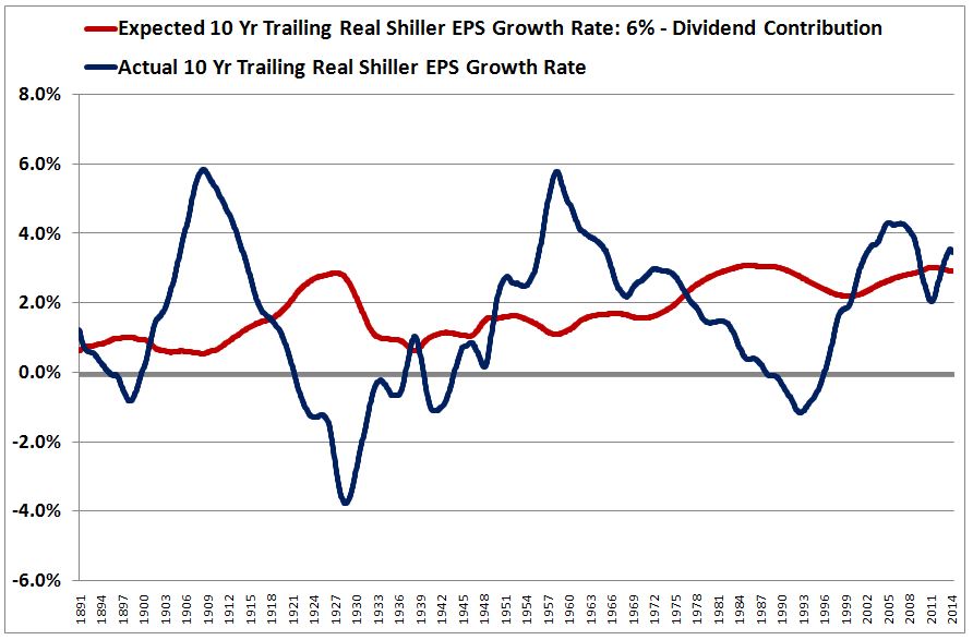
The following chart illustrates the trailing magnitude of this error from 1891 to 2014. The blue line is the actual realized 10 year trailing Shiller EPS growth rate. The red line is the 10 year trailing Shiller EPS growth rate that would have been expected, given the dividend’s return contribution.
As you can see, the blue and red lines frequently deviate. To illustrate the impact of the deviation, the following chart shows the sum (black line) of the trailing 10 year return contributions from growth (gold) and dividends (green) from 1891 to 2014.
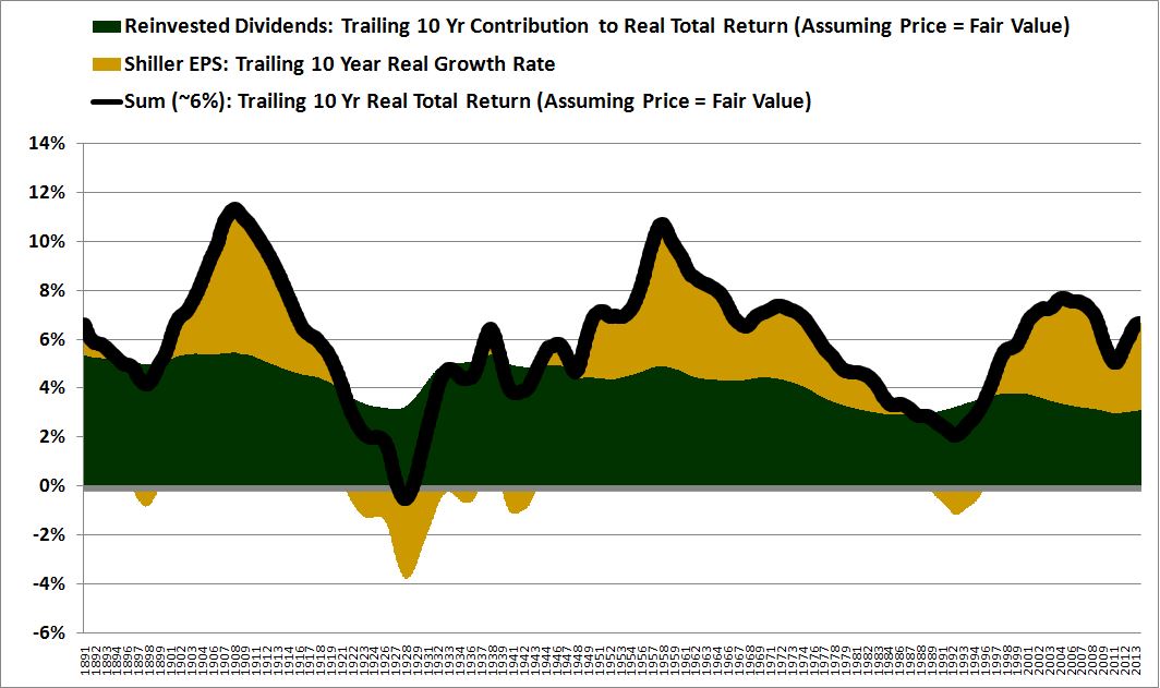
As you can see, the growth contribution on a 10 year horizon (yellow) is highly variable, despite relatively stable dividend contributions. The consequence of this variability is that the method’s total return estimates, based on a nice, neat 6% assumption, frequently turn out to be wrong.
For a concrete example, suppose that you try to use the method to estimate 10 year real total returns from November 1948 to November 1958. Your estimate will be way off, even though the CAPE ended the period almost exactly at the mean value of 17. The reason your estimate will be off is that corporate performance during the period was unusually strong, reflecting, in part, the high productivity growth and pent-up demand that was unleashed into the post-war economy. From November 1948 to November 1958, the real growth rate of the Shiller EPS was an abnormally high 6%, versus the 1% that the model would have predicted based on the dividend contribution. The actual return contribution from the sum of growth and dividends was 11%, versus the 6% that the model uses.
Given the depressed starting point of the CAPE in November 1948 (around 10), the method’s estimate of the future 10 year return was 11%. But the actual 10 year return that ensued was a whopping 17%, even though the method’s assumption that CAPE would mean-revert to 17 turned out to be true. The following chart highlights the large deviation.
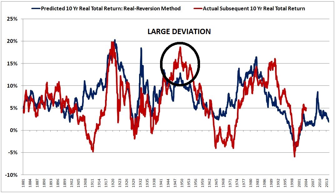
Note that “Shillerization” of the returns cannot eliminate the deviation, because the deviation is driven by errors associated with a variable that is already a “Shillerization” of sorts–Shiller’s 10 year average of inflation-adjusted EPS. As a general rule, Shillerization only works for errors associated with excursions that are brief relative to the Shillerization time horizon. This error is not brief, but persists over a multi-decade period.
It turns out that the only way to eliminate the deviation is to use a longer time horizon. In practice, the method’s 6% assumption doesn’t hold over 10 year periods–there’s too much 10 year variability in corporate performance across history. It only holds over very long periods–north of, say, 40 years.
The following chart shows the trailing 10 year and the trailing 40 year Shiller EPS growth rate errors from 1921 to 2014 (actual Shiller EPS growth rate minus model-expected Shiller EPS growth rate given the contribution of dividends):
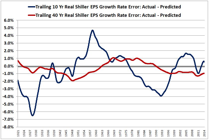
As you can see, using a longer time horizon pulls the error (red line) down towards zero, rendering the 6% assumption, and the method in general, more reliable.
The following chart shows the sum (black line) of the growth (gold) and dividend (green) contributions from 1921 to 2014 using a trailing 40 year horizon instead of a trailing 10 year horizon:
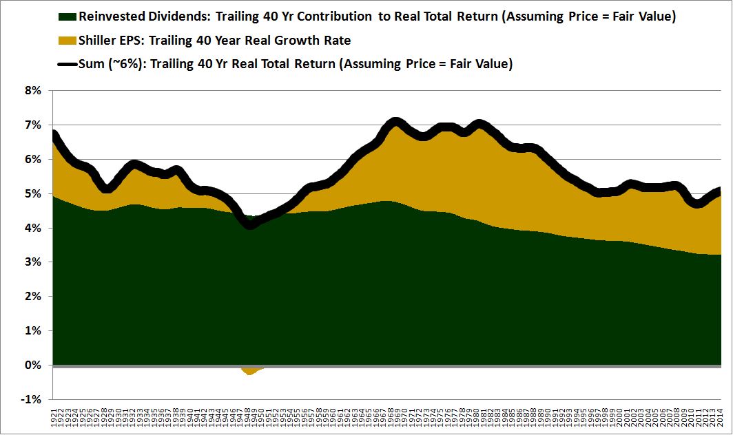
As you can see, on a trailing 40 year horizon, the black line gets much closer to a consistent 6%. It stays roughly within 1% of that value across the entire period, minimizing the error.
To return to the previous 1948-1958 example, if you use the method to predict the return over the trailing 40 years instead of the trailing 10 years–starting in November of 1918 instead of 1948–you dilute the 1948-1958 anomaly with three decades worth of additional economic data. The 6% assumption ends up being significantly closer to the actual sum of the growth and dividend contributions, which from 1918 to 1948 turned out to be 5.3%.
Now, let’s look at the second source of error, variabilities in the valuations at which dividends are reinvested. This error rarely gets noticed, but it matters. In a recent piece, I gave a concrete example of how powerful it can be–over the long-term, it’s capable of rendering a permanent 66% market crash more lucrative for existing investors than a permanent 200% market melt-up (assuming, of course, that the crash and the melt-up are driven by changes in valuation, rather than changes in actual earnings).
Recall that our method rested on the assumption that dividends are reinvested in the market at “fair value”, defined as true book value, which we took to correspond to a Shiller CAPE equal to the long-term average. This assumption is obviously wrong. Markets frequently trade at depressed and elevated levels, which means that dividends are frequently reinvested at higher and lower implied rates of return–sometimes over long periods of time, in ways that don’t net out to zero.
Interestingly, even if periods of high and low valuation were to be perfectly matched over time, their net effect on the returns associated with reinvested dividends would still be greater than zero. To illustrate with a concrete example, suppose that the market spends 5 years at a price of 100, and 5 years at a price of 50. The mean is 75. Suppose that the implied return at that mean is 6%, consistent with earlier assumptions. The bidirectional excursion will actually boost the return above 6%. For 5 years, dividends will be reinvested at a price of 100–which, simplistically, is an implied return of 4.5%. For another 5 years, dividends will be reinvested at a price of 50–which, simplistically, is an implied of 9%. These two deviations, when combined, do not average to the 6% mean. Rather, they average to 6.75%. The 9% period earned a return 3% higher than the mean, whereas the 4.5% period earned a return only 1.5% below the mean. When combined, the two deviations do not fully cancel. We can see, then, that symmetric price volatility around the mean actually boosts total returns relative to the norm.
The following chart shows the effect that reinvesting dividends at market prices rather than “fair value” has had on 10 year real total returns, from 1891 to 2014:
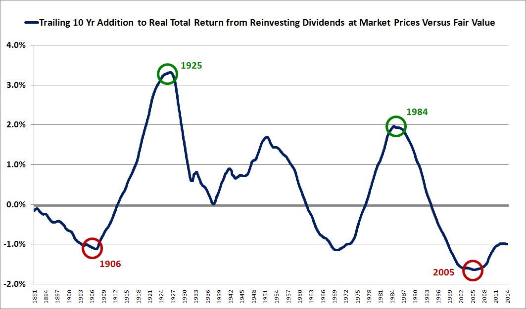
(Details: We calculate the effect by creating two “fake” real total return indices. In the first index, we set prices equal to “fair value”, a Shiller CAPE equal to the historic average of 15.3. We reinvest dividends at those prices. In the second index, we set prices equal to “fair value”, but we reinvest the dividends at whatever the actual market price happened to be. The chart shows the difference between the trailing 10 year annualized returns of each index.)
Notice that if we look backwards from 1925 and 1984 (circled in green), the effect added a healthy 3% and 2% to the real total return respectively. That’s because the markets in the ten years preceding 1925 and 1984 were very cheap–they traded at average CAPEs in the single digits. Dividends were reinvested into those cheap markets, earning abnormally high rates of return.
At the other extreme, if we look backwards from 1906 and 2005 (circled in red), the effect added -1% and -1.5% to the actual real total return respectively, reflecting the fact that the markets in the ten years that preceded 1906 and 2005 were expensive–with the former trading at an average CAPE near 20 (despite a high dividend payout ratio), and the latter trading at an average CAPE north of 30. Dividends were reinvested into those expensive markets, earning abnormally low rates of return.
As before, the only way to reduce the effect that this error–the error of assuming that dividends are always reinvested at fair value, when they are not–will have on our method is to extend the time horizon. 10 years is too short, there’s too much variability in the average valuations seen across different 10 year historical periods. As the chart below illustrates, when we use a longer time horizon, 40 years (red), we successfully dilute the impact of the variability.
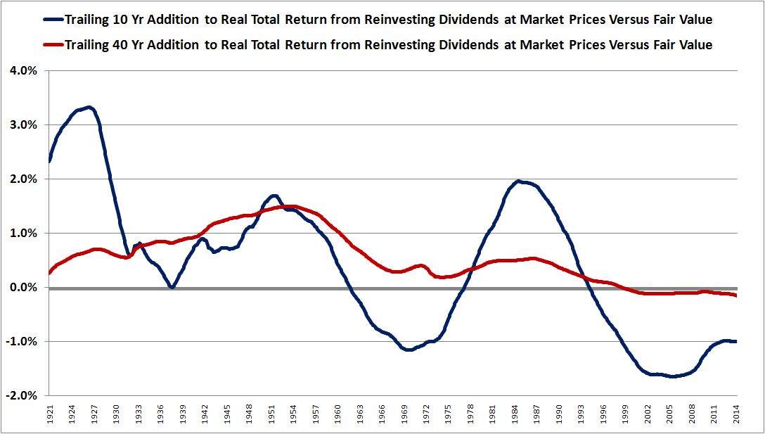
The extension of the horizon to 40 years dilutes the outlier periods and flattens out the net error towards zero. In the 40 year period from 1925 back to 1885, the extreme cheapness of the late 1910s and early 1920s is mixed in with the expensiveness seen at the turn of the 19th century, when the CAPE was well above 20 (despite a very high payout ratio). In the 40 year period from 2005 back to 1965, the extreme expensiveness of the tech bubble and its aftermath is mixed in with the extreme cheapness of the bear markets of the late 1970s and early 1980s, where the CAPE traded in the single digits.
Notice that both lines have trended lower across the full period–that’s because, on trailing 10 year and 40 year average horizons, equity valuations, as measured by the CAPE, have trended towards becoming more expensive. Notice also that the average value of both lines is greater than zero. This is due, in part, to the fact that symmetric price volatility has a positive net effect on the reinvested dividend’s contribution. It does not cancel out.
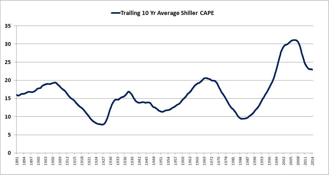
This brings us to the third source of error in the method, the most obvious one–the fact that the volatile Shiller CAPE often spends significant amounts of time far away from its assumed mean of 17. This error has been especially acute in recent times. Over the last 23 years, the Shiller CAPE hasn’t even come close to reverting to its assumed mean–it’s only spent 4% of the time at or below it. Regardless of the reasons why the Shiller CAPE has failed to revert to its assumed mean, the fact remains that it hasn’t–consequently, the method hasn’t reliably worked to predict returns. It’s missed the mark, dramatically.
Unfortunately, not even Shillerization can solve this recent problem. That’s because the 10 year averages of CAPE over the last two decades are just as elevated as the spot values. The following chart shows the trailing 10 year average CAPE from 1891 to 2014.
To manage the problem, all that we can really do is increase the time horizon. 10 years is hopeless, but 40 years might have a chance. Superficially, it can spread the error out over a larger period of time, shrinking the error on an annualized basis. In general, as time horizons get longer, valuations have a smaller annual impact on future returns–albeit a smaller annual impact imposed over more years. In the infinite limit, valuation has an infinitesimally small impact–but an infinitesimally small impact imposed over an infinity of years.
Alternatively, we could extend the Shillerization time span from 10 years to something larger, like 3o or 40 years (whatever is needed to adequately dilute out the shift in the CAPE seen over the last 23 years). But, from a testing standpoint, this approach would be highly suspicious. Method doesn’t work? No problem, just make the Shillerization time span as big as you need it to be in order to dilute out the periods of history that are causing problems. The approach would also eliminate a huge chunk of data from the analysis. We would run out of actual realized returns to measure the method’s predictions against at 39 + 40 = 79 years ago, 1925. So our effective sample period wouldn’t even reach WW2 as a starting point.
We don’t want our backtest of the method to devolve into one great big “averaging” of all of history. On that approach, the correlation between predicted and actual returns will end up being high simply because we will be working with a small sample size of predictions and realized results (as the time horizon increases, the pool of realized returns to compare the predictions with decreases), and because both the predictions and the realized results will have been massively smoothed over decades and decades into numbers that converge on the average, 6%, regardless of the starting valuation. Strong results in such a backtest will prove nothing, at least nothing of value to present investors.
If our point is to say that the CAPE is higher than its long-term historical average, we should say this, and then stop. It’s higher than its long-term historical average, period, proceed as you wish. Showing that we can use the CAPE to predict long-term returns if they are Shillerized across enormous periods of time, three or four decades, doesn’t say anything more.
Spectacular Long-Term Predictions: The Tricks of the Trade
The following chart shows the performance of the “Shillerized” metric on a 40 year time horizon, comparing the average of future annual 40, 41, 42, …, 49 year return predictions to the average of the actual subsequent annual returns over the next 40, 41, 42, …, 49 years.
Bullseye–we’ve nailed it, a near perfect hit. The correlation rises to 0.92. Note that this is a correlation across all 133 years of available data, all 1,584 months–not some arbitrarily chosen sample that coincidentally happens to fit well with the author’s desired conclusions. Of note, the method gets the prediction wrong in the late 1940s and early 1950s–this is because the subsequent returns in those years ended in the late 1990s and early 2000s, a period where the CAPE was dramatically elevated, and where even a “Shillerization” of the results couldn’t save the method from its incorrect mean-reversion assumptions. But we’ll be reasonable and let that error slide.
Now, to the fun part. We’re going to look under the hood to see what’s actually going on in this chart. When we do that, we’re going to discover numerous other “hidden” places where the method failed, but where coincidences bailed it out, contributing to the illusion of the robust fit seen above.
We saw earlier that even on 40 year horizons, the assumption of a 6% normal real return from growth and dividends was not fully accurate. The post-war period up to the 1980s, for example, exhibited a number above 7%; the pre-war period up to the late 1940s exhibited a number closer to 4%.
We also know that the Shiller CAPE has been substantially elevated, not just from the late 1990s to the early 2000s, but for the entirety of the last 23 years, from 1991 until today, save for a few brief months during the financial crisis. A 10 year “Shillerization” of prices and returns should not be enough to dilute out the powerful impact of that deviation.
So what gives? Where did those errors and deviations go? Why don’t they appear as errors and deviations in the chart? To answer the question, we need to plot the errors alongside each other. Then, everything will become crystal clear.
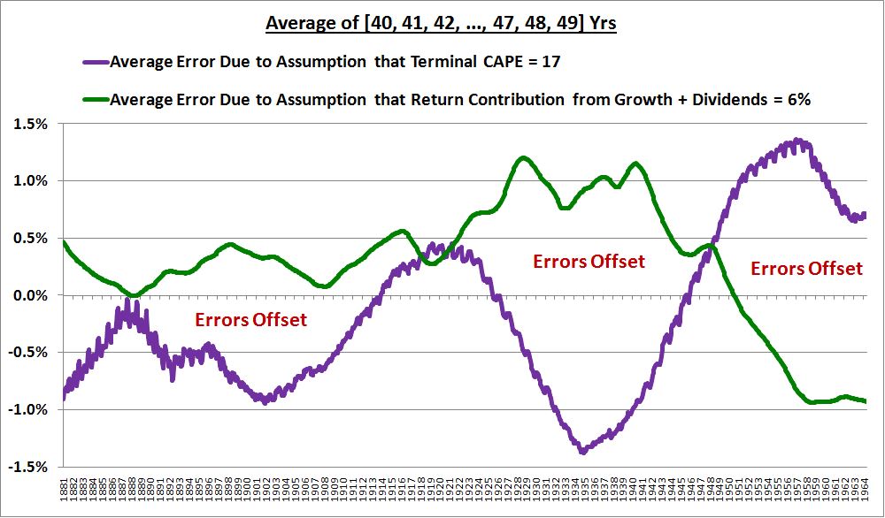
The following chart shows the actual “Shillerized” errors in the “6% growth plus dividends” assumption and in the “Terminal CAPE = 17” assumption, on a subsequent 40 to 49 year horizon, for each month from 1881 to the most recent realized data point.
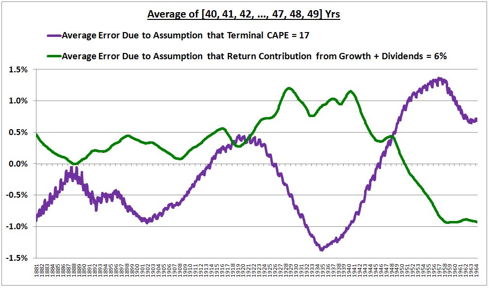
(Details: The green line is the difference between (1) the average of what the actual subsequent 40, 41, 42, …, 49 year annual real returns ended up being, and (2) the average of what those annual real returns would have been if the final CAPE had been 17, per the model’s assumptions. The purple line is the difference between (1) the average of the actual realized sums of the real return contribution from Shiller EPS growth and dividends reinvested at market prices over the subsequent 40, 41, 42, …, 49 years, and (2) what the model assumed those sums should have been–6%.)
Now, look closely at the chart. What’s interesting about it? The purple line and the green line are 180 degrees out of phase. Therefore, they cancel each other out. That’s why the curve fits so well, despite the persistent errors.
To prove that we’re calculating the errors correctly, the following chart shows the predicted error, given the deviations in the two assumptions (of a 6% normal real return, and a terminal CAPE of 17), alongside the actual error (the difference between the actual return that occurred in the market and the return that the model predicted would occur). The two track each other almost perfectly.
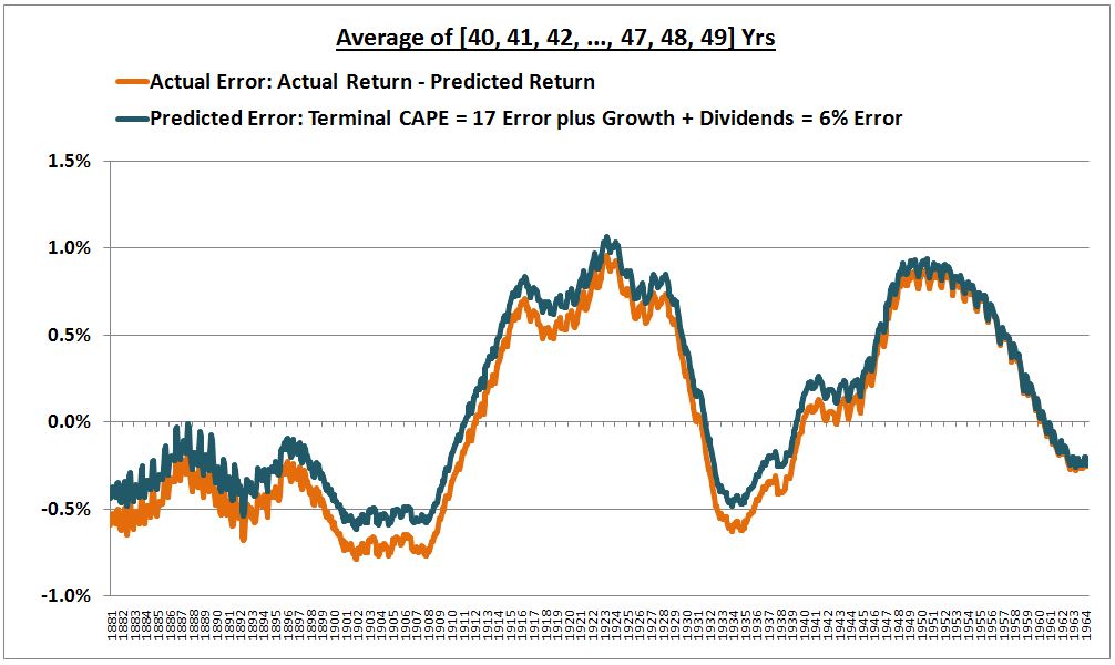
(Details: Here we’re calculating the “Terminal CAPE = 17” error by taking the difference between what the annualized real price return actually was over the horizon, and what it would have been if the CAPE had ended up being 17, as the method assumed. We’re calculating the “Growth + Dividends = 6% Error” by subtracting 6% from the sum of–(a) the real Shiller EPS growth that actually occurred, (b) the dividend return that would have occured if dividends were reinvested at fair value, and (c) the effect of reinvesting dividends at market prices instead of fair value.)
The following chart shows the errors alongside the actual and predicted returns from 1881 to the most recent realized data point:
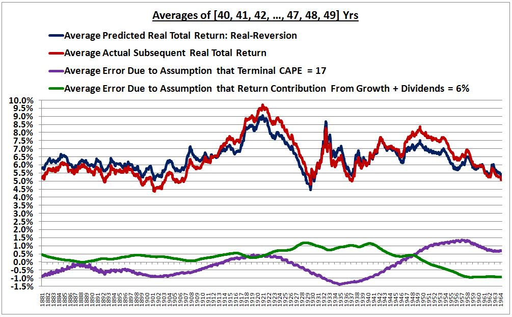
Notice that whenever the sum of the purple and green lines is positive–for example, from around 1914 to around 1929, and from around 1947 to around 1958–the red line, the actual return, exceeds the blue line, the predicted return. Whenever the sum of the purple and green lines is negative–for example, from around 1881 to around 1911–the blue line, the predicted return, exceeds the red line, the actual return. For most of the period, the sum is reasonably close to zero, creating the perception of a robust fit.
Now, before we launch allegations of curve-fitting–i.e., building a fit out of coincidental patterning that cannot be trusted to hold out of sample–we need to ask, is there a potential relationship between these two errors, a story we can tell to connect them? If the answer is yes, then maybe the method is capturing something real. Maybe it’s predictions should be trusted.
Here’s one interesting story we can tell: lower than normal growth (negative green lines) leads to lower than normal interest rates, which leads to higher than normal Shiller CAPEs (positive purple lines), and vice versa. If this story is true, then the method is capturing a real relationship in the data, and the robustness of the fit shouldn’t be discounted.
Stories are easy to tell, and hard to refute. Fortunately, in this case, we have a simple way to test them. Just change the time horizon. Surely, if the method can predict returns on a 40 year time horizon, it should be able to predict them on, say, a 60 year time horizon. Any convenient error-cancelling relationship that the method exploits should not be unique to just 40 years–it should apply across all sufficiently long time horizons.
So let’s look at a 60 year time horizon instead. The following chart shows the performance of the metric on a 60 year “Shillerized” time horizon, comparing the average of future annual 60, 61, 62, …, 69 year return predictions to the average of the actual subsequent annual returns over the next 60, 61, 62, …, 69 years.
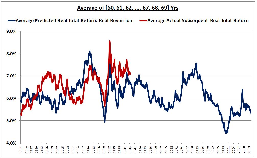
Lo and behold, the fit devolves into a mess. The correlation falls from 0.92 to 0.40. What happened? Ultimately, the errors that just so happened to cancel on a 40 year time horizon ceased to cancel on a 60 year horizon. It may look like the predictions do OK–the maximum deviation between predicted and actual is only around 1%. But that’s 1% per year over 70 years. And we’ve Shillerized the returns. Clearly, the fit is unacceptable.
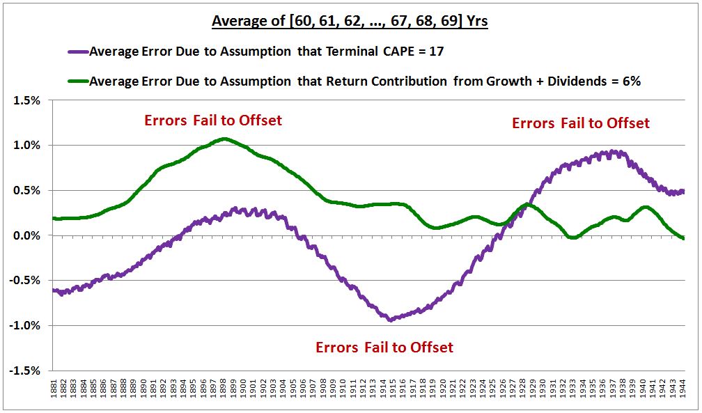
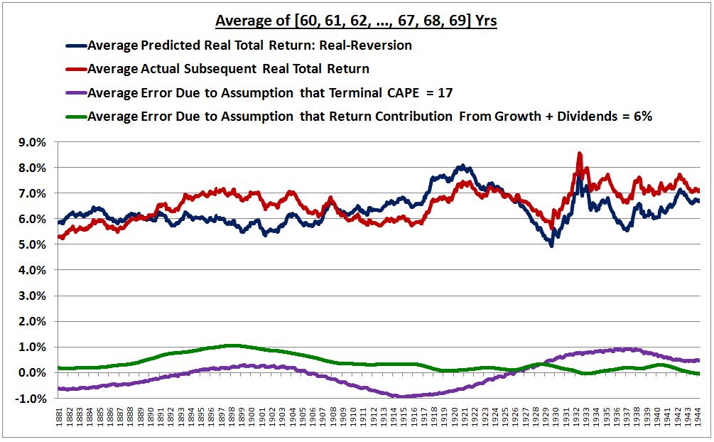
What we have, then, is de facto proof of a curve-fit. When you change the time horizon appreciably, the fit unravels. The following chart shows the two errors alongside the actual and predicted returns.
Now–and this is the key takeaway–every single forecasting method in existence that purports to use valuation to accurately predict point-to-point equity market returns in U.S. historical data exploits this same trick. The data set that we’re working with, covering the U.S. equity market from 1871 to 2014, contains significant variability in the average valuations and average rates of return that it exhibits. That variability can be dampened by limiting the analysis to very large time horizons and by using Shillerization, but it can’t be eliminated. It’s been especially pronounced in the last two decades, with valuations having migrated to what might otherwise be described as a “permanently high plateau.” Given this migration, any model that attempts to predict returns in the data set on the basis of a normal rate of return is bound to produce significant errors, even when the returns are Shillerized. The only way for the predictions of the model to fit with the actual results in the presence of the errors is for the errors to cancel. When you see a tight fit, that’s always what’s happening.
When a person sits behind a computer and sifts through different configurations of a model (different prediction time horizons, different mean valuations, different growth rate assumptions, different date ranges for testing, etc.) to find the configuration in which the predictions best “fit” with the actual subsequent results, that person is unwittingly “selecting out” the configuration that, by chance, happens to best achieve the necessary cancellation of the model’s errors. The result ends up being inherently biased. For this reason, we should be deeply skeptical of models that claim to reliably predict returns in historical data on the basis of successful in-sample testing. We should judge them not by the superficial accuracy of their fits (an accuracy that is almost always engineered), but by the accuracy of their underlying assumptions.
Mean-reversion methods make the assumption that non-cyclical valuation metrics will eventually fall from their “permanently high plateaus” of the last two decades down to their prior long-term averages–with respect to the the Shiller CAPE, the assumption is that the metric is going to fall from 26.5 to 17. Is that assumption going to prove true? Forget the curve-fits, forget the backtests, forget the data-mining, and just examine the assumption itself. If it’s going to prove true, and if the normal return would otherwise be 6% real, then the actual return will be 1.4% real. If it isn’t going to prove true, then the return will be something else.
Final Results and Conclusion
Here are the full performance results for “Real-Reversion”, with starting points in 1881 and 1935 (post-Depression, effective post-Gold-Standard):
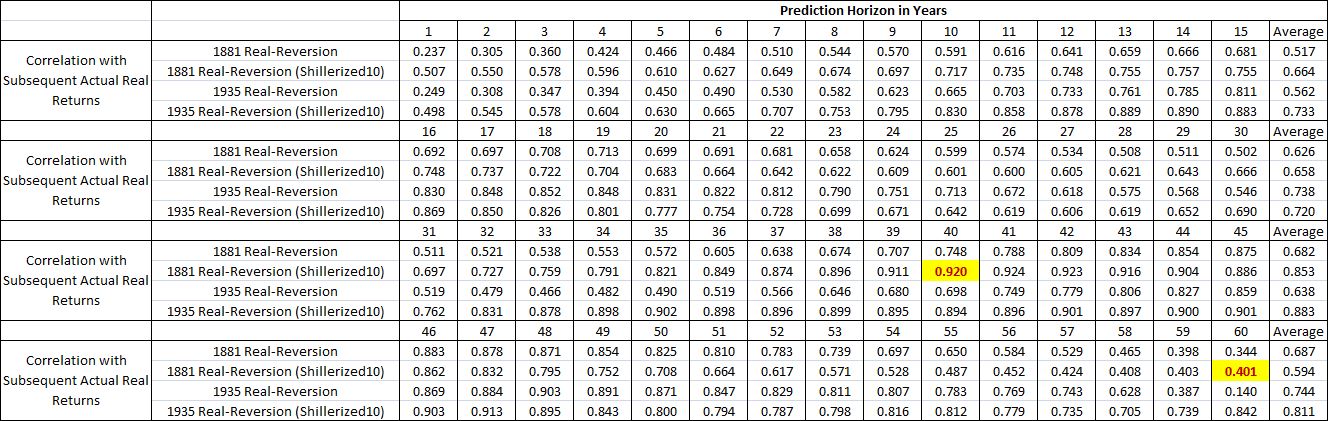
Across the full spectrum of time horizons, the correlation just isn’t very strong. That’s because valuations aren’t reliably mean-reverting. There’s too much valuation variability in the historical data set, even when we use “Shillerized” averages over 10 year time spans. For the correlation to get tight, the growth and dividend errors have to superficially cancel with the valuation errors–but that doesn’t consistently happen, hence the breakdown.
Now, to be clear, I’m not saying that valuation doesn’t matter. Valuation definitely matters–its power as a return factor has been demonstrated in stock markets all over the world. Holding other factors constant, if you buy cheap, you’ll do better, on average, than if you buy expensive. This is true whether we’re talking about individual stocks, or the aggregate market.
What I’m taking issue with is the notion that we can use valuation to build “historically reliable” prediction models whose specific predictions closely align with actual past results, models that give us warrant to attach special “scientific” or “empirical” privilege to our bullish or bearish opinions. That, we cannot do. Given the significant variability in the historical data set, the best we can do is mine curve-fits whose errors conveniently offset and whose deviations conveniently disappear. These are not worth the effort.
In the end, valuation metrics are only capable of giving us a crude idea of what future returns will be. In the present context, they can tell us what we already know and accept: that future real returns will be less than the 6% historical average (a perfectly appropriate outcome that we should expect at equilibrium, given the secular decline in interest rates and the below-average implied returns on the assets that most directly compete with equities: cash and bonds). But they can’t tell us much more. They can’t arbitrate the debate between those of us who expect, say, 3% real returns for U.S. equities going forward, and who therefore judge the market to be fairly valued (relative to cash at a likely negative long-term real return), and those of us who expect negative real returns for equities, and who therefore find the market to be egregiously overvalued. The reason valuations can’t arbitrate that debate is that they don’t reliably mean-revert. If they did, we wouldn’t be having this discussion.