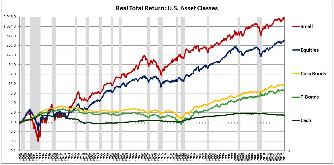
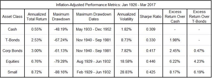
Looking back at asset class performance over the course of market history, we notice a hierarchy of excess returns. Small caps generated excess returns over broad equities, which generated excess returns over corporate bonds, which generated excess returns over treasury bonds, which generated excess returns over treasury bills (cash), and so on. This hierarchy is illustrated in the chart and table below, which show cumulative returns and performance metrics for the above asset classes from January 1926 to March 2017 (source: Ibbotson, CRSP).
(Note: To ensure a fair and accurate comparison between equities and fixed income asset classes, we express returns and drawdowns in real, inflation-adjusted terms. We calculate volatilities and Sharpe Ratios using real absolute monthly returns, rather than nominal monthly returns over treasury bills.)
The observed hierarchy represents a puzzle for the efficient market hypothesis. If markets are efficient, why do some asset classes end up being priced to deliver such large excess returns over others? An efficient market is not supposed to allow investors to generate outsized returns by doing easy things. Yet, historically, the market allowed investors to earn an extra 4% simply by choosing equities over long-term bonds, and an extra 2% simply by choosing small caps inside the equity space. What was the rationale for that?
The usual answer given is risk. Different types of assets expose investors to different levels of risk. Risk requires compensation, which is paid in the form of a higher return. The additional 4% that equity investors earned over bond investors did not come free, but represented payment for the increased risk that equity investing entails. Likewise, the 2% bonus that small cap investors earned over the broad market was compensation for the greater risk associated with small companies.
A better answer, in my view, is that investors didn’t know the future. They didn’t know that equity earnings and dividends were going to grow at the pace that they did. They didn’t know that small cap earnings and dividends were going to grow at an even faster pace. They didn’t know that inflation was going to have the detrimental long-term effects on real bond returns that it had. And so on. Amid this lack of future knowledge, they ended up pricing equities to outperform bonds by 4%, and small caps to outperform the broad market by 2%. Will we see a similar outcome going forward? Maybe. But probably not.
Let’s put aside the question of whether differences in “risk”, whatever that term is used to mean, can actually justify the differences in excess returns seen in the above table. In what follows, I’m going to argue that if they can, then as markets develop and adapt over time, those excess returns should fall. Risk assets should become more expensive, and the cost of capital paid by risk issuers should come down.
The argument is admittedly trivial. I’m effectively saying that improvements in the way a market functions should lead to reductions in the costs that those who use it–those who seek capital–should have to pay. Who would disagree? Sustainable reduction in issuer cost is precisely what “progress” in a market is taken to mean. Unfortunately, when we flip the point around, and say that the universe of risk assets should grow more expensive in response to improvements, people get concerned, even though the exact same thing is being said.
To be clear, the argument is normative, not descriptive. It’s an argument about what should happen, given a certain assumption about the justification for excess returns. It’s not an argument about what actually has happened, or about what actually will happen. As a factual matter, on average, the universe of risk assets has become more expensive over time, and implied future returns have come down. The considerations to be discussed in this piece may or may not be responsible for that change.
We tend to use the word “risk” loosely. It needs a precise definition. In the current context, let “risk” refer to any exposure to an unattractive or unwanted possibility. To the extent that such an exposure can be avoided, it warrants compensation. Rational investors will demand compensation for it. That compensation will typically come in the form of a return–specifically, an excess return over alternatives that successfully avoid it, i.e., “risk-free” alternatives.
We can arbitrarily separate asset risk into three different types: price risk, inflation risk, and fundamental risk.
Price Risk and Inflation Risk
Suppose that there are two types of assets in the asset universe.
(1) Zero Coupon 10 Yr Government Bond, Par Value $100.
(2) Cash Deposited at an Insured Bank — expected long-term return, 2%.
The question: What is fair value for the government bond?
The proper way to answer the question is to identify all of the differences between the government bond and the cash, and to then settle on a rate of return (and therefore a price) that fairly compensates for them, in total.
The primary difference between the government bond and the cash is that the cash is liquid. You can use it to buy things, or to take advantage of better investment opportunities that might emerge. Of course, you can do the same with the government bond, but you can’t do it directly. You have to sell the bond to someone else. What will its price in the market be? How will its price behave over time? You don’t know. When you go to actually sell it, the price could end up being lower than the price you paid for it, in which case accessing your money will require you to accept a loss. We call exposure to that possibility price risk. The bond contains it, cash does not. To compensate, the bond should offer an excess return over cash, which is the “price-risk-free” alternative.
To fully dismiss the price risk in a government bond investment, you would have to assume total illiquidity in it. Total illiquidity is an extreme cost that dramatically increases the excess return necessary to draw an investor in. That said, price risk is a threat to more than just your liquidity. It’s a threat to your peace of mind, to your measured performance as an investor or manager, and to your ability to remain in leveraged trades. And so even if you have no reason to want liquid access to your money, no reason to care about illiquidity, the risk that the price of an investment might fall will still warrants some compensation.
A second category of risk is inflation risk. Inflation risk is exposure to the possibility that the rate of inflation might unexpectedly increase, reducing the real value of a security’s future payouts. The cash is offering payouts tied to the short-term rate, which (typically) gets adjusted in response to changes in inflation. It therefore carries a measure of protection from that risk. The bond, in contrast, is offering a fixed payout 10 years from now, and is fully exposed to the risk. To compensate for the difference, the bond should offer an excess return over cash.
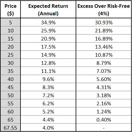
Returning to the scenario, let’s assume that you assess all of the differences between the bond and cash, to include the bond’s price risk and inflation risk, and conclude that a 2% excess return in the bond is warranted. Your estimate of fair value, then, will be $67.55, which equates to a 4% yield-to-maturity (YTM).
Fundamental Risk: An Introduction to Lotto Shares
A security is a stream of cash flows and payouts. Fundamental risk is risk to those cash flows and payouts–the possibility that they might not pay out. We can illustrate its impact with an example.
In the previous scenario, you estimated fair value for the government bond to be $67.55, 4% YTM. Let’s assume that you’re now forced to invest your entire net worth into either that bond at that price, or into a new type of security that’s been introduced into the market, a “Lotto Share.”
To reiterate, your choice:
(1) Zero Coupon 10 Yr Government Bonds, 4% YTM, Price $67.55, Par Value $100.
(2) Zero Coupon 10 Yr Lotto Shares, Class “A”.
Lotto Share: A government bond with a random payout. Lotto Shares are issued in separate share classes. At the maturity date of each share class, the government flips a fair coin. If the coin ends up heads (50% chance), the government exchanges each outstanding share in the share class for a payment of $200. If the coin ends up tails (50% chance), the government makes no exchange, and each outstanding share in the share class expires worthless.
Before you make your choice, note that the Lotto Shares being offered all come from the same class, Class “A.” All of their payouts will therefore be decided by the same single coin flip, to take place at maturity 10 years from now.
The question: What is fair value for a Lotto Share?
To answer the question, try to imagine that you’re actually in the scenario, forced to choose between the two options. What price would Lotto Shares have to sell at in order for you to choose to invest in them? Would $67.55 be appropriate? How about $50? $25? $10? $5? $1? One penny? Is there any price that would interest you?
It goes without saying that your answer will depend on whether you can diversify among the two options. Having the entirety of your portfolio, or even a sizeable portion thereof, invested in a security that has a 50% chance of becoming worthless represents an enormous risk. You would need the prospect of an enormous potential reward in order to take it–if you were willing to take it at all. But if you have the option to invest much smaller portions of your portfolio into the security, if not simply for the “fun” of doing so, the potential reward won’t need to be as large.
Assume that you do have the ability to diversify between the two options. The question will then take on a second dimension: allocation. At each potential price for Lotto Shares, ranging from zero to infinity, how much of your portfolio would you choose to allocate to them?
Let’s assume that Lotto Shares are selling for the same price as normal government bonds, $67.55. How much of your portfolio would you choose to put into them? If you’re like most investors, your answer will be 0%, i.e., nothing. To understand why, notice that Lotto Shares have the same expected (average) payout as normal government bonds, $100 ($200 * 50% + $0 * 50% = $100). The difference is that they pay that amount with double-or-nothing risk–at maturity, you’re either going to receive $200 or $0. That risk requires compensation–an excess return–over the risk-free alternative. Lotto Shares priced identically to normal government bonds (the risk-free alternative) do not offer such compensation, therefore you’re not going to want to allocate anything to them. You’ll put everything in the normal government bond.
Now, in theory, we can envision specific situations where you might actually want double-or-nothing risk. For example, you might need lifesaving medical treatment, and only have half the money needed to cover the cost. In that case, you’ll be willing to make the bet even without compensation–just flip the damn coin. If it comes back heads, you’ll survive, if it comes back tails… who cares, you would have died anyways. Alternatively, you might be managing other people’s money under a perverse “heads-you-win, tails-they-lose” incentive arrangement. In that case, you might be perfectly comfortable submitting the outcome to a coin flip, without receiving any extra compensation for the risk–it’s not a risk to you. But in any normal, healthy investment situation, that’s not going to be the case. Risk will be unwelcome, and you won’t willingly take it on unless you get paid to do so.
Note that the same point holds for price risk and inflation risk. Prices can go up in addition to down, and inflation can go down in addition to up. You can get lucky and end up benefitting from having taken those risks. But you’re not a gambler. You’re not going to take them unless you get compensated.
The price and allocation question, then, comes down to a question of compensation: at each level of potential portfolio exposure, what expected (or average) excess return over the risk-free alternative (i.e., normal government bonds) is necessary to compensate for the double-or-nothing risk inherent in Lotto Shares? The following table lists the expected 10 year annualized excess returns for Lotto Share at different prices. Note that these are expected returns. They’re only going to hold on average–in actual practice, you’re going to get double-or-nothing, because the outcome is going to be submitted to only one flip.
We can pose the price and allocation question in two different directions:
(1) (Allocation –> Price): Starting with an assumed allocation–say, 40%–we could ask: what price and excess return for Lotto Shares would be needed to get you to allocate that amount, i.e., risk that amount in a coin flip?
(2) (Price –> Allocation): Starting with an assumed price–say, $25, an annual excess return of 10.87%–we could ask: how much of your portfolio would you choose to allocate to Lotto Shares, if offered that price?
Up to now, we’ve focused only on fundamental risk, i.e., risk to a security’s cash payouts. In a real world situation, we’ll need to consider price risk. As discussed earlier, price risk requires compensation in the form of an excess return over the “price-risk-free” alternative, cash. But notice that in our scenario, we don’t have the option of holding cash. Our options are to invest in Lotto Shares or to invest in normal government bonds. The factor that requires compensation, then, is the difference in price risk between these two options.
Because Lotto Shares carry fundamental risk, their price risk will be greater than the price risk of normal government bonds. As a general rule, fundamental risk creates its own price risk, because it forces investors to grapple with the murky question of how that risk should be priced, along with the even murkier question of how others in the market will think it should be priced (in the Keynesian beauty contest sense). Additionally, as normal government bonds approach maturity, their prices will become more stable, converging on the final payment amount, $100. As Lotto Shares approach maturity, the opposite will happen–their prices will become more volatile, as more and more investors vacillate on whether to stay in or get out in advance of the do-or-die coin flip.
That said, price risk is not the primary focus here. To make it go away as a consideration, let’s assume that once we make our initial purchases in the scenario, the market will close permanently, leaving us without any liquidity in either investment. We’ll have to hold until maturity. That would obviously be a disadvantage relative to a situation where we had liquidity and could sell, but the disadvantage applies equally to both options, and therefore cancels out of the pricing analysis.
Returning to the question of Lotto Share pricing, for any potential investor in the market, we could build a mapping between each possible price for a Lotto Share, and the investor’s preferred allocation at that price. Presumably, at all prices greater than $67.55 (the price of the normal government bond), the investor’s preferred allocation will be 0%. As the price is reduced below that price, the preferred allocation will increase, until it hits a ceiling representing the maximum percentage of the portfolio that the investor would be willing to risk in a coin flip, regardless of how high the potential payout might be. The mappings will obviously be different for different investors, determined by their psychological makeups and the specific financial and life circumstances they are in.
I sat down and worked out my own price-allocation mapping, and came up with the table shown below. The first column is the Lotto Share price. The second column is my preferred allocation at that price. The third and fourth column are the absolute dollar amounts of the excess gains (on heads) and excess losses (on tails) that would be received or incurred if a hypothetical $1,000,000 portfolio were allocated at that percentage:
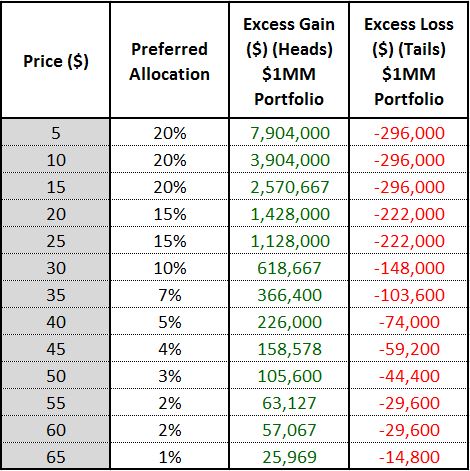
Working through the table, if I were managing my own $1,000,000 portfolio, and I were offered a Lotto Share price of $65, I would be willing to invest 1%, which would entail risking $14,800 in a coin flip to make $25,969 on heads. If I were offered a price of $40, I would be willing to invest 5%, which would entail risking $74,000 in a coin flip to make $226,000 on heads. If I were offered $15, I would be willing to invest 20%, which would entail risking $296,000 in a coin flip to make $2,750,667 on heads. And so on.
Interestingly, I found myself unwilling to go past 20%. To put any larger amount at risk, I would need the win-lose odds to be skewed in my favor. In Lotto Shares, they aren’t–they’re even 50/50. What’s skewed in my favor is the payout if I happen to win–that’s very different.
The example illustrates the extreme impact that risk-aversion has on asset valuation and asset allocation. To use myself as an example, you could offer me a bargain basement price of $5 for a Lotto Share, corresponding to a whopping 35% expected annual return over 10 years, and yet if that expected return came with double-or-nothing risk attached, I wouldn’t be willing to allocate anything more than a fifth of my assets to it.
Interestingly, when risk is extremely high, as it is with Lotto Shares, the level of interest rates essentially becomes irrelevant. Suppose that you wanted to get me to allocate more than 20% of my portfolio to Lotto Shares. To push me to invest more, you could drop the interest rate on the government bond to 2%, 0%, -2%, -4%, -6%, and so on–i.e., try to “squeeze” me into the Lotto Share, by making the alternative look shitty. But if I’m grappling with the possibility of a 50% loss possibility on a large portion of my portfolio, your tiny interest rate reductions will make no difference at all to me. They’re an afterthought. That’s why aggressive monetary policy is typically ineffective at stimulating investment during downturns. To the extent that investors perceive investments to be highly risky, they will require huge potential rewards to get involved. Relative to those huge rewards, paltry shifts in the cost of borrowing or in the interest rate paid for doing nothing will barely move the needle.
I would encourage you to look at the table and try to figure out how much you would be willing to risk at each of the different prices. If you’re like me, as you grapple with the choice, you will find yourself struggling to find a way to get a better edge on the flip, or to somehow diversify the bet. Unfortunately, given the constraints of the scenario, there’s no way to do either.
Interestingly, if the price-allocation mapping of all other investors in the market looked exactly like mine, Class “A” Lotto Shares would never be able to exceed 20% of the total capitalization of the market. No matter how much it lowered the price, the government would not be able to issue any more of them beyond that capitalization, because investors wouldn’t have any room in their portfolios for the additional risk.
Adding New Lotto Share Classes to the Market
Let’s examine what happens to our estimate of the fair value of Lotto Shares when we add new share classes to the market.
Assume that three new share classes are added, so that the we now have four –“A”, “B”, “C”, “D”. Each share class matures in 10 years, and pays out $200 or $0 based on the result of a single coin flip. However, and this is crucial, each share class pays out based on its own separate coin flip. The fundamental risk in each share class is therefore idiosyncratic–independent of the risks in the other share classes.
To summarize, then, you have to invest your net worth across the following options:
(1) Zero Coupon 10 Yr Government Bonds, 4% YTM, Price $67.55, Par Value $100.
(2) Zero Coupon 10 Yr Lotto Shares, Class “A”.
(3) Zero Coupon 10 Yr Lotto Shares, Class “B”.
(4) Zero Coupon 10 Yr Lotto Shares, Class “C”.
(5) Zero Coupon 10 Yr Lotto Shares, Class “D”.
The question: What is fair value for a Lotto Share in this scenario?
Whatever our fair value estimate happens to be, it should be the same for all Lotto Shares in the market, given that those shares are identical in all relevant respects. Granted, if the market supplies of the different share classes end up being different, then they might end up trading at different prices, similar to the way different share classes of preferred stocks sometimes trade at different prices. But, as individual securities, they’ll still be worth the same, fundamentally.
Obviously, if you choose to allocate to Lotto Shares in this new scenario, you’re going to want to diversify your exposure equally across the different share classes. That will make the payout profile of the investment more attractive. Before, you only had one share class to invest in–Class “A”. The payout profile of that investment was a 50% chance of $200 (heads) and a 50% chance of $0 (tails). If you add a new share class to the mix, so that you have an equal quantity of two in the portfolio, your payout will be determined by two coin flips instead of one–a coin flip that decides your “A” shares and a coin flip that decides your “B” shares. On a per share basis, the payout profile will then be a 25% chance of receiving $200 (heads for “A”, heads for “B”), a 50% chance of receiving $100 (heads for “A”, tails for “B” or tails for “B”, heads for “A”), and a 25% chance of receiving $0 (tails for “A”, tails for “B”). If you add two more shares classes to the mix, so that you have an equal quantity of four in the portfolio, the payout profile will improve even further, as shown in the table below.
(Note: The profile follows a binomial distribution.)
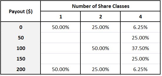
In the previous scenario, the question was, what excess return over normal government bonds would Lotto Shares need to offer in order to get you to invest in them, given that the investment has a 50% chance of paying out $200 and a 50% chance of paying out $0? With four share classes in the mix, the question is the same, except that the investment, on a per share basis, now has a 6.25% chance of paying out $0, a 25% chance of paying out $50, a 37.5% chance of paying out $100, a 25% chance of paying out $150, and a 6.25% chance of paying out $200. As before, the expected payout is $100 per share. The difference is that this expected payout comes with substantially reduced risk. Your risk of losing everything in it, for example, is longer 50%. It’s 6.25%, a far more tolerable number.
Obviously, given the significant reduction in the risk, you’re going to be willing to accept a much lower excess return in the shares to invest in them, and therefore you’ll be willing to pay a much higher price. In a way, this is a very surprising conclusion. It suggests that the estimated fair value of a security in a market can increase simply by the addition of other, independent securities into the market. If you have an efficient mechanism through which to diversify across those securities, you won’t need to take on the same risk in owning each individual one. But that risk was precisely the basis for there being a price discount and an excess return in the shares–as it goes away, the discount and excess return can go away.
In the charts below, we show the payout profiles for Lotto Share investments spread equally across 100, 1,000, and 10,000 different Lotto Share Classes. As you can see, the distribution converges ever more tightly around the expected (average) $100 payout per share.
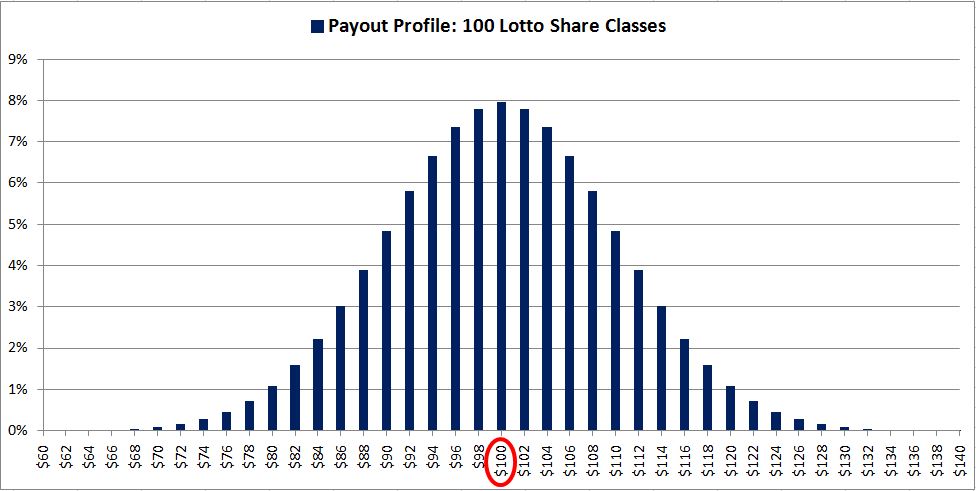
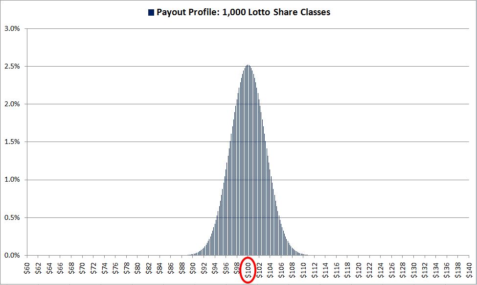
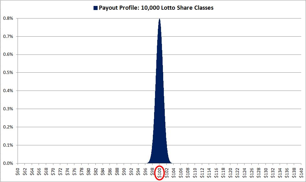
As you can see from looking at this last chart, if you can invest across 10,000 independent Lotto Shares, you can effectively turn your Lotto Share investment into a normal government bond investment–a risk-free payout. In terms of the probabilities, the cumulative total payout of all the shares (which will be determined by the number of successful “heads” that come up in 10,000 flips), divided by the total number of shares, will almost always end up equaling a value close to $100, with only a very tiny probabilistic deviation around that number. In an extreme case, the aggregate payout may end up being $98 per share or $102 per share–but the probability that it will be any number outside that is effectively zero. And so there won’t be any reason for Lotto Shares to trade at any discount relative to normal government bonds. The excess returns that had to be priced into them in earlier scenarios where their risks couldn’t be pooled together will be able to disappear.
Equities as Lotto Shares
Dr. Hendrik Bessembinder of Arizona State University recently published a fascinating study in which he examined the return profiles of individual equity securities across market history. He found that the performance is highly positively skewed. Most individual stocks perform poorly, while a small number perform exceptionally well. The skew is vividly illustrated in the chart below, which shows the returns of 54,015 non-overlapping samples of 10 year holding periods for individual stocks:
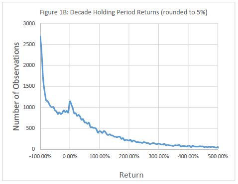
The majority of stocks in the sample underperformed cash. Almost half suffered negative returns. A surprisingly large percentage went all the way down to zero. The only reason the market as a whole performed well was because a small number of “superstocks” generated outsized returns. Without the contributions of those stocks, average returns would have been poor, well below the returns on fixed income of a similar duration. To say that individual stocks are “risky”, then, is an understatement. They’re enormously risky.
As you can probably tell, our purpose in introducing the Lotto Shares is to use them to approximate the large risk seen in individual equity securities. The not-so-new insight is that by combining large numbers of them together into a single equity investment, we can greatly reduce the aggregate risk of that investment, and therefore greatly reduce the excess return needed to compensate for it.
This is effectively what we’re doing when we go back into the data and build indices in hindsight. We’re taking the chaotic payout streams of individual securities in the market (the majority of which underperformed cash) and merging them together to form payout streams that are much smoother and well-behaved. In doing so, we’re creating aggregate structures that carry much lower risk than the actual individual securities that the actual investors at the time were trading. The fact that it may have been reasonable for those investor to demand high excess returns over risk-free alternatives when they were trading the securities does not mean that it would be similarly reasonable for an investor today, who has the luxury of dramatically improved market infrastructure through which to diversify, to demand those same excess returns.
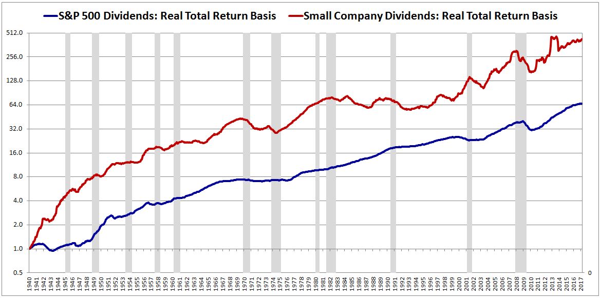
When we say that stocks should be priced to deliver large excess returns over long-term bonds because they entail much larger risks, we need to be careful not to equivocate on that term, “risk”. The payouts of any individual stock may carry large risks, but the payouts of the aggregate universe of stocks do not. As the chart below shows, the aggregate equity payout is a stream of smooth, reasonably well-behaved cash flows, especially when the calamity of the Great Depression (a likely one-off historical event) is bracketed out.
(Note: We express the dividend stream on a real total return basis, assuming each dividend is reinvested back into the equity at market).

In terms of stability and reliability, that stream is capable of faring quite well in a head-to-head comparison with the historical real payout stream of long-term bonds. Why then, should it be discounted relative to bonds at such a high annual rate, 4%?
A similar point applies to the so-called “small cap” risk premium. As Bessembinder’s research confirms, individual small company performance is especially skewed. The strict odds of any individual small company underperforming, or going all the way to zero, is very high–much higher than for large companies. Considered as isolated individual investments, then, small companies merit a substantial price discount, a substantial excess return, over large companies. But when their risks are pooled together, the total risk of the aggregate goes down. To the extent that investors have the ability to efficiently invest in that aggregate, the required excess return should come down as well.
The following chart shows the historical dividend stream (real total return basis) of the smallest 30% of companies in the market alongside that of the S&P 500 from January 1928 to March 2017:
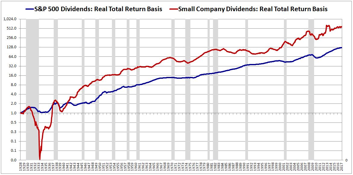
Obviously, pooling the risks of individual small caps together doesn’t fully eliminate the risk in their payouts–they share a common cyclical risk, reflected in the volatility of the aggregate stream. If we focus specifically on the enormous gash that took place around the Great Depression, we might conclude that a 2% discount relative to large caps is appropriate. But when we bracket that event out, 2% starts to look excessive.
Progress in Diversification: Implications for the Cost of Capital
In the earlier scenarios, I told you up front that each class of Lotto Shares has a 50% chance of paying out $200. In an actual market, you’re not going to get that information so easily. You’re going to have to acquire it yourself, by doing due diligence on the individual risk asset you’re buying. That work will translate into time and money, which will subtract from your return.
To illustrate, suppose that there are 10,000 Lotto Share Classes in the market: “A”, “B”, “C”, “D”, “E”, etc. Each share class pays out P(A), P(B), P(C), P(D), P(E), etc., with independent probabilities Pr(A), Pr(B), Pr(C), Pr(D), Pr(E), etc. Your ability to profitably make an investment that diversifies among the different share classes is going to be constrained by your ability to efficiently determine what all of those numbers are. If you don’t know what they are, you won’t have a way to know what price to pay for the shares–individually, or in a package.
Assume that it costs 1% of your portfolio to determine each P and Pr for an individual share class. Your effort to put together a well-diversified investment in Lotto Shares, an investment whose payout mimics the stability of the normal government bond’s payout, will end up carrying a large expense. You will either have to pay that expense, or accept a poorly diversified portfolio, with the increased risk. Both disadvantages can be fully avoided in a government bond, and therefore to be willing to invest in the Lotto Share, you’re going to need to be compensated. As always, the compensation will have to come in the form of a lower Lotto Share price, and a higher return.
Now, suppose that the market develops mechanisms that allows you to pool the costs of building a diversified Lotto Share portfolio together with other investors. The cost to you of making a well-diversified investment will come down. You’ll therefore be willing to invest in Lotto Shares at higher prices.
Even better, suppose that the investment community discovers that it can use passive indexing strategies to free-load on the fundamental Lotto Share work that a small number of active investors in the market are doing. To determine the right price to pay, people come to realize that they can drop all of the fretting over P, Pr, and so on, and just invest across the whole space, paying whatever the market is asking for each share–and that they won’t “miss” anything in terms of returns. The cost of diversification will come down even further, providing a basis for Lotto Share prices to go even higher, potentially all the way up to the price of a normal government bond, a price corresponding to an excess return of 0%.
The takeaway, then, is that as the market builds and popularizes increasingly cost-effective mechanisms and methodologies for diversifying away the idiosyncratic risks in risky investments, the price discounts and excess returns that those investments need to offer, in order to compensate for the costs and risks, comes down. Very few would dispute this point in other economic contexts. Most would agree, for example, that the development of efficient methods of securitizing mortgage lending reduces the cost to lenders of diversifying and therefore provides a basis for reduced borrowing costs for homeowners–that’s its purpose. But when one tries to make the same argument in the context of stocks–that the development of efficient methods to “securitize” them provides a basis for their valuations to increase–people object.
In the year 1950, the average front load on a mutual fund was 8%, with another 1% annual advisory fee added in. Today, given the option of easy indexing, investors can get convenient, well-diversified exposure to many more stocks than would have been in a mutual fund in 1950, all for 0%. This significant reduction in the cost of diversification warrants a reduction in the excess return that stocks are priced to deliver, particularly over safe assets like government securities that don’t need to be diversified. Let’s suppose with all factors included, the elimination of historical diversification costs ends up being worth 2% per year in annual return. Parity would then suggest that stocks should offer a 2% excess return over government bonds, not the historical 4%. Their valuations would have a basis to rise accordingly.
Now, to clarify. My argument here is that the ability to broadly diversify equity exposure in a cost-effective manner reduces the excess return that equities need to offer in order to be competitive with safer asset classes. In markets where such diversification is a ready option–for example, through low-cost indexing–valuations deserve to go higher. But that doesn’t mean that they actually will go higher. Whether they actually will go higher is not determined by what “deserves” to happen, but by what buyers and sellers actually choose to do, what prices they agree to transact at. They can agree to transact at whatever prices they want.
The question of whether the increased availability and popularity of equity securitization has caused equity valuations to go higher is an interesting question. In my view, it clearly has. I would offer the following chart as circumstantial evidence.
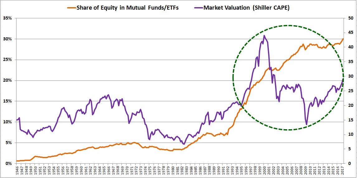
Notice the large, sustained valuation jump that took place in the middle of the 1990s. Right alongside it, there was a large, sustained jump in the percentage of the equity market invested through mutual funds and ETFs. Correlation is not causation, but there are compelling reasons to expect a relationship in this case. Increased availability and popularity of vehicles that allow for cheap, convenient, well-diversified market exposure increases the pool of money inclined to bid on equities as an asset class–not only during the good times, but also when buying opportunities arise. It’s reasonable to expect that the result would be upward pressure on average valuations across the cycle, which is exactly what we’ve seen.
History: The Impact of Learning and Adaptation
One problem with using Lotto Shares as an analogy to risk assets, equities in particular, is that Lotto Shares have a definite payout P and a definite probability Pr that can be known and modeled. Risk assets don’t have that–the probabilities around their payouts are themselves uncertain, subject to unknown possibility. That uncertainty is risk–in the case of equities, it’s a substantial risk.
If we’re starting out from scratch in an economy, and looking out into the future, how can we possibly know what’s likely to happen to any individual company, or to the corporate sector as a whole? How can we even guess what those probabilities are?
But as time passes, a more reliable recorded history will develop, a set of known experiences to consult. As investors, we’ll be able to use that history and those experiences to better assess what the probabilities are, looking out into the future. The uncertainty will come down–and with it the excess return needed to justify the risks that we’re taking on.
We say that stocks should be expensive because interest rates are low and are probably going to stay low forever. The rejoinder is: “Well, they were low in the 1940s and 1950s, yet stocks weren’t expensive.” OK, but so what? Why does that matter? All it means is that, in hindsight, investors in the 1940s and 1950s got valuations wrong. Should we be surprised?
Put yourself in the shoes of an investor in that period, trying to determine what the future for equities might look like. You have the option of buying a certain type of security, a “stock”, that pays out company profits. In the aggregate, do you have a way to know what the likely growth rates of those profits will be over time? No. You don’t have data. You don’t have a convenient history to look at. Consequently, you’re not going to be able to think about the equity universe in that way. You’re going to have to stay grounded at the individual security level, where the future picture is going to be even murkier.
In terms of price risk, this is what the history of prices will look like from your vantage point:
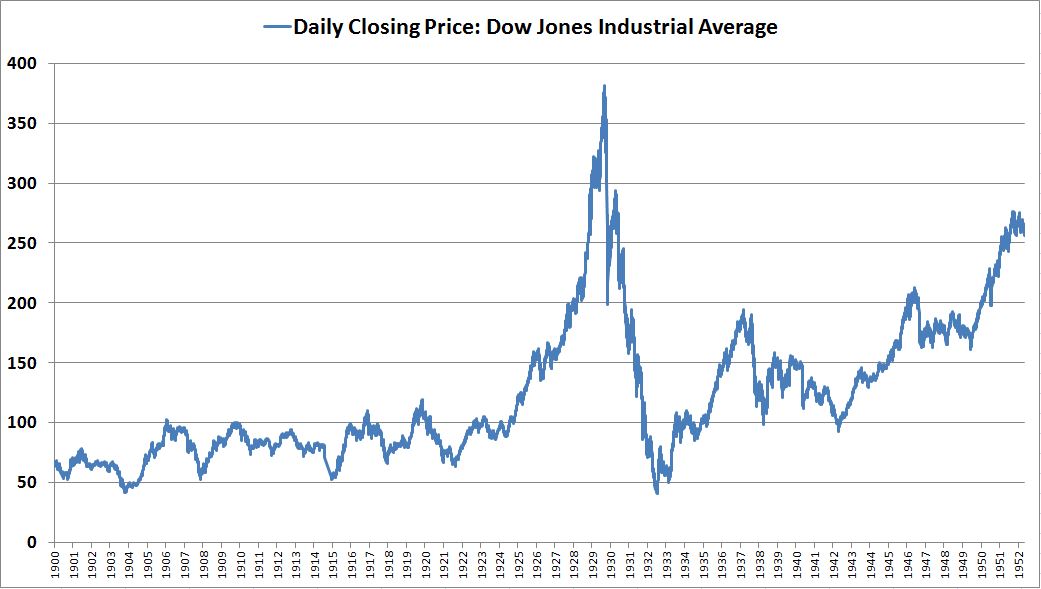
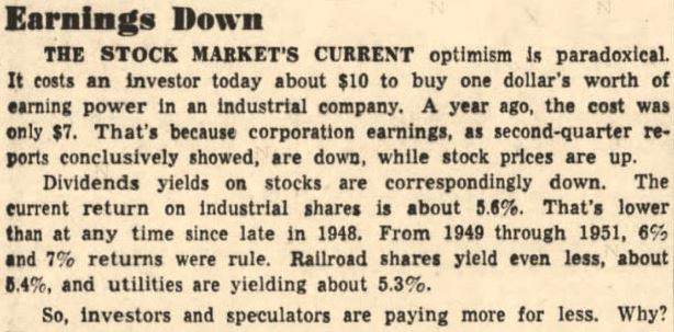
Judging from the chart, can you reliably assess the risk of a large upcoming drop? Can you say, with any confidence, that if a drop like the one that happened 20 odd years ago happens again, that it will be recovered in due course? Sure, you might be able to take solace in the fact that the dividend yield, at 5.5%, is high. But high according to who? High relative to what? The yield isn’t high relative to what it was just a few years ago, or to what it was after the bubble burst. One can easily envision cautious investors pointing that out to you. Something like this, taken right out of that era:
Now, fast forward to the present day. In terms of estimating future growth rates and returns on investment, you have the chart below, a stream of payouts that, on a reinvested basis, has grown at a 6% average real rate over time, through the challenges of numerous economic cycles, each of which was different in its own way. Typical investors may not know the precise number, but they’re aware of the broader historical insight, which is that equities offer the strongest long-term growth potential of any asset class, that they’re where investors should want to be over the long haul: “Stocks For The Long Run.” That insight has become ingrained in the financial culture. One can say that its prevalence is just another symptom of the “bubble” that we’re currently in, but one has to admit that there’s at least some basis for it.
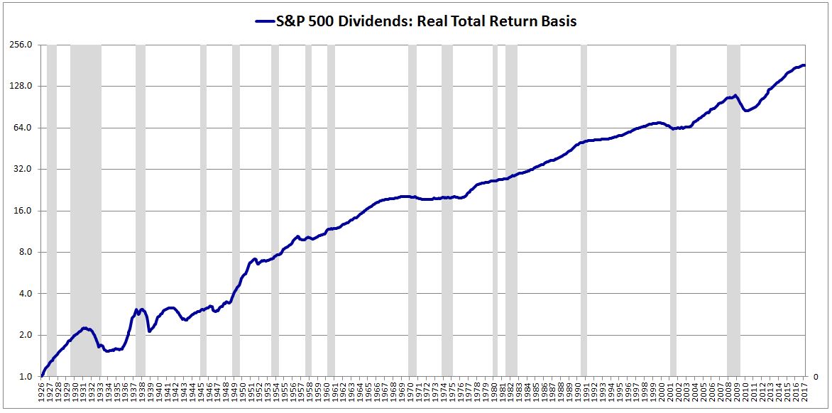
Now, I’ll be the first to acknowledge that the 6% number is likely to be lower going forward. In fact, that’s the whole point–equity returns need to be lower, to get in line with the rest of the asset universe. The mechanism for the lower returns, in my view, is not going to be some kind of sustained mean-reversion to old-school valuations, as the more bearishly inclined would predict. Rather, it’s going to come directly from the market’s expensiveness itself, from the fact that dividend reinvestments, buybacks and acquisitions will all be taking place at much higher prices than they did in the past. On the assumption that current valuations hold, I estimate that long-term future returns will be no more than 4% real. To get that number, I recalculate the market’s historical prices based on what they would have been if the market had always traded at its current valuation–a CAPE range of 25 to 30. With the dividends reinvested at those higher prices, I then calculate what the historical returns would have been. The answer: 4% real, reflecting the impact of the more expensive reinvestment, which leads to fewer new shares purchased, less compounding, and a lower long-term return. Given the prices current investors are paying, they have little historical basis for expecting to earn any more than that. If anything, they should expect less. The return-depressing effect of the market’s present expensiveness is likely to be amplified by the fact that there’s more capital recycling taking place today–more buybacks, acquisitions, etc., all at expensive prices–and less growth-producing real investment. So 4% represents a likely ceiling on returns, not a floor.
Regardless of the specific return estimate that we settle on, the point is, today, the facts can be known, and therefore things like this can be realistically modeled–not with anything close to certainty, but still in a way that’s useful to constrain the possibilities. Investors can look at a long history of US equity performance, and now also at the history of performance in other countries, and develop a picture of what’s likely to happen going forward. In the distant past, investors did not have that option. They had to fly blind, roll the dice on this thing called the “market.”
In terms of price risk, this is what your rear view mirror looks like today:
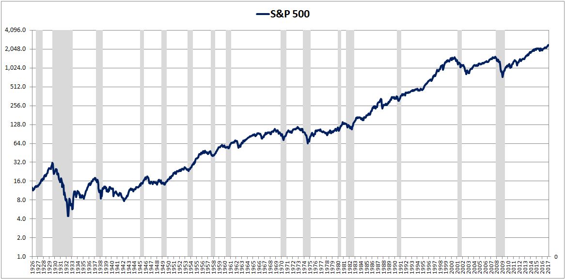
Sure, you might get caught in a panic and lose a lot of money. But history suggests that if you stick to the process, you’ll get it back in due course. That’s a basis for confidence. Importantly, other investors are aware of the same history that you’re aware of, they’ve been exposed to the same lessons–“think long-term”, “don’t sell in a panic”, “stocks for the long run.” They therefore have the same basis for confidence that you have. The result is a network of confidence that further bolsters the price. Panics are less likely to be seen as reasons to panic, and more likely to be seen as opportunities to be taken advantage of. Obviously, panics will still occur, as they must, but there’s a basis for them to be less chaotic, less extreme, less destructive than they were in market antiquity.
Most of the historical risk observed in U.S. equities is concentrated around a single event–the Great Depression. In the throes of that event, policymakers faced their own uncertainties–they didn’t have a history or any experience that they could consult in trying to figure out how to deal with the growing economic crisis. But now they do, which makes it extremely unlikely that another Great Depression will ever be seen. We saw the improved resilience of the system in the 2008 recession, an event that had all of the necessary ingredients to turn itself into a new Great Depression. It didn’t–the final damage wasn’t even close to being comparable. Here we are today, doing fine.
An additional (controversial) factor that reduces price risk relative to the past is the increased willingness of policymakers to intervene on behalf of markets. Given the lessons of history, policymakers now have a greater appreciation for the impact that market dislocations can have on an economy. Consequently, they’re more willing to actively step in to prevent dislocations from happening, or at least craft their policy decisions and their communications so as to avoid causing dislocations. That was not the case in prior eras. The attitude towards intervention was moralistic rather than pragmatic. The mentality was that even if intervention might help, it shouldn’t happen–it’s unfair, immoral, a violation of the rules of the game, an insult to the country’s capitalist ethos. Let the system fail, let it clear, let the speculators face their punishments, economic consequences be damned.
To summarize: over time, markets have developed an improved understanding of the nature of long-term equity returns. They’ve evolved increasingly efficient mechanisms and methodologies through which to manage the inherent risks in equities. These improvements provide a basis for average equity valuations to increase, which is something that has clearly been happening.