The recent piece on the dangers of backtesting has attracted an unusual amount of attention for a piece on this blog. I’d like to thank everyone who read and shared the piece, and also those who offered up commentary on it.
To be clear, my intent in presenting the Daily Momentum example was not to challenge the Fama-French-Asness momentum factor in specific, or the phenomenon of momentum in general. Obviously, one failed version of a momentum strategy would not be sufficient to refute the mountain of evidence, both empirical and theoretical, that exists in support of the phenomenon. My intent was simply to show, in an entertaining way, that robust patterns backed by extremely large amounts of historical data can spontaneously weaken and disappear, out of the blue. The fact that the example involved momentum per se was incidental.
As investors, we do not intentionally search the data to find “fallen” strategies–strategies that worked for long periods of time, and that then stopped working. When we encounter such strategies, we discard them, because they are useless to us. What we try to find are “successful” strategies–strategies that have worked consistently across the relevant periods of history, and that have not yet failed in the data.
If we did search specifically for “fallen” strategies, we would come to realize that there are more of them in the data than there are “successful” strategies. Statistically, the odds are therefore good that when we do find a “successful” strategy, that what we’ve actually found is a strategy that is going to become a “fallen” strategy, as the future plays out. We need to take that risk seriously, and engage the process of quantitative research with an appropriate level of skepticism.
To many, I’m probably stating the obvious–but the point is not obvious to everyone. It certainly was not obvious to me when I was first introduced to the fun and exciting process of trying to use a computer to solve the puzzles of financial markets.
Slip: The Validity of a Counterfactual
To conserve space in the prior piece, I left out a discussion of an interesting philosophical question. When we conduct a backtest, should we use a slip equal to what the bid-ask spread was at the time, or should we use a slip equal to what the bid-ask spread will be now, when we actually run the strategy in the real world? In the context of the example, if it’s 1999, and I’m testing Daily Momentum to determine whether or not I should implement it as a timing strategy in a real portfolio, should I apply a slip equal to the current bid-ask spread of the security that I am going to use in the strategy, or should I apply a slip equal to the actual bid-ask spread that existed in the market during the years that I’m backtesting across–in this case, the years 1928 to 1999?
The market’s bid-ask spread in past eras was very wide, much wider than today, where it’s almost non-existent in many securities. As the following chart shows, the average spread from 1928 to 1999 was north of .60%, a number that would have completely destroyed any strategy that traded daily–and that would have significantly impaired strategies that traded monthly or even quarterly.  The price quoted in a historical time series for a stock or an index is typically the midpoint between the highest bid and the lowest ask. Importantly, that price is not a price that any investor ever had access to. If an investor wanted to sell, she did not have the option of selling at the “midpoint”–she had to sell at the bid. If she wanted to buy, she did not have the option of buying at the “midpoint”–she had to buy at the ask.
To give a specific example, if a time series for the stock of “Caterpillar Tractor” shows a price of 4.75 on June 15th, 1932, that number, 4.75, is not an actual price that anyone could have transacted at. Rather, it is the midpoint between (1) the best ask price that buyers could have transacted at, which was 5, and (2) the best bid price that sellers could have transacted at, which was 4 1/2, quoted in that fraction.
To correct for the difference between the quoted price and the actual transactable price in the backtest, we apply a slip. Unfortunately, when we apply a slip that reflects the current bid-ask spread, rather than the historical bid-ask spread, we effectively allow our backtest to trade at mythical prices, prices that no one that was actually present in the market had any ability to trade at.
In the Caterpillar Tractor example, if we use a 0.10% slip, we are letting our model buy Caterpillar Tractor for 4.755, when no one was actually offering to sell shares at that price. Similarly, we are letting our model sell Caterpillar Tractor for 4.745, when no one was actually offering to buy shares at that price. This approach, if we were to use it, would obviously be inauthentic. If our strategy were to perform well, we would not be able to accurately say:
“An investor would have outperformed using our strategy.”
Rather, we would have to say:
“If an investor could have traded at a price that didn’t actually exist, to a buyer or seller that was not actually willing to buy or sell at that price, then the investor would have outperformed using our strategy.”
If that’s what “success” in a backtest means, it’s hard to walk away impressed.
A backtest that transacts using the market’s current spread rather than its historical spread relies on a counterfactual–an assumed hypothetical state of affairs that did not actually exist. This reliance alone, of course, is not the issue. All backtests rely on counterfactuals–the very concept of a backtest requires us to assume that someone did something that no one actually did, i.e., executed a specific trade at a specific price in a specific amount. The issue is whether the assumed counterfactual is compatible with the historical pattern that the tested strategy exploits. And that’s where our use of a current bid-ask spread, rather than a historical one, gets us into trouble.
For a 0.10% bid-ask spread to have existed in the past, that spread would have had to have been profitable to market makers. And for the spread to have been profitable to market makers–profitable enough for them to accept the risk to their capital of offering it–the market would have had to have seen dramatically increased levels of volume. But if the market of the past had seen dramatically increased levels of volume, would it have gone on to produce the same Daily Momentum pattern that it actually produced? Can we be sure that the increased volume–or any other perturbation that might have been required for a tighter spread–would have left the pattern unaffected?
The answer is no. And therefore if we want our backtest of Daily Momentum, or of any strategy that exploits a technical price pattern, to be maximally reliable, we need to commit to applying a slip that matches the actual spread in place at the time. For most of the pre-1990s period, this means a slip of 0.60% or above, applied to each round-trip transaction.
With that said, even though, in a strict sense, the slip assumptions in the backtest are inaccurate and cast signficant doubt on the successful implementation of the strategy, the weird price pattern that the strategy exploits is very real, and demands an explanation. Moreover, the example still serves its intended purpose, which was to show that a seemingly robust pattern can persist in a market or an economy for a very long time, and then disappear.
The “Stale Price” Effect: Daily Momentum and Index Exaggerations
Cliff Asness, whose thoughts on the topic of momentum are obviously worth far more than mine, especially considering that he was among those who discovered the phenomenon (when I was still in middle school), offered a brilliant explanation for part of the success of Daily Momentum. Historically, not all stocks have traded on every market trading day. Some stocks experienced days of zero volume, driven either by illiquidity or suspensions.
The fact that not all stocks traded on every market trading day gives an artificial advantage to momentum strategies. If an index goes up on a given day, a momentum strategy will buy the index, or at least be more likely to buy it. If, inside the index, there are stocks that did not trade on that day, those stocks will remain quoted at stale prices–either yesterday’s price, or a price from the last day that a trade occurred or a quote was taken. The stale prices will then feed into the index price. A momentum strategy, in buying the index at the quoted index price, will effectively get to buy the untraded stocks at their stale prices. Tomorrow, or some time in the future, when the stocks do trade again, their prices will rise to reflect the market’s upward movement on the missed trading day. The momentum strategy, having bought the stocks at stale prices, will then register a profit–a profit that’s entirely fake and unattainable, but that nonetheless shows up as real in the backtest.
In testing, we find that daily momentum beats 2-day momentum beats 3-day momentum beats 4-day momentum and so on. This observed ranking of the performances supports the view that Cliff’s effect–which, for convenience, we can name the “stale price” effect–is driving the result. All else equal, shorter horizon momentum strategies would be expected to perform better than longer horizon strategies because they leverage the “stale price” effect to a greater degree. They trade more frequently, and therefore they register the effect’s gains more frequently.
The “stale price” effect allows for an elegant explanation of the decay and eventual implosion of Daily Momentum’s historical performance. Recall that the question we were unable to answer in the prior piece was: why did the performance start to weaken in the 1980s and 1990s, and then implode in the 2000s? What was the cause of the loss of efficacy? We now have a potentially compelling answer: the cause was an increase in the broadness of stock market volume, provoked by the widespread adoption of technologically-assisted investment vehicles that trade all securities indiscriminately–index futures, index mutual funds, index ETFs, and so on. Broader stock market volume, brought about by these changes, would have reduced the “stale price” effect, removing a key driver of the strategy’s outperformance.
It turns out that we can assess the impact of the “stale price” effect by backtesting Daily Momentum on individual stocks. If we get rid of indices, and just backtest the individual names themselves, we will have removed the effect altogether. The strategy’s subsequent performance will then reveal what the effect’s true impact was.
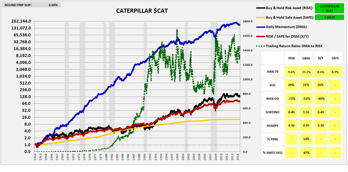
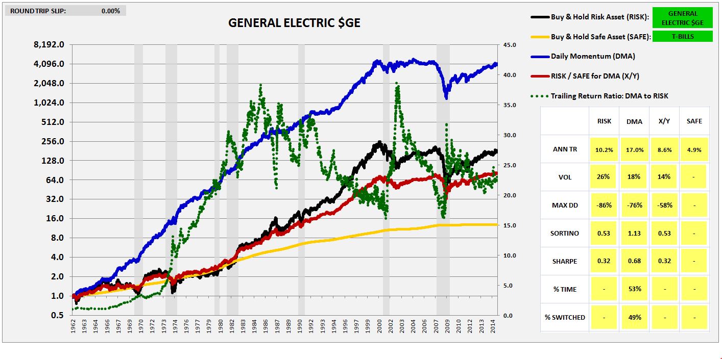
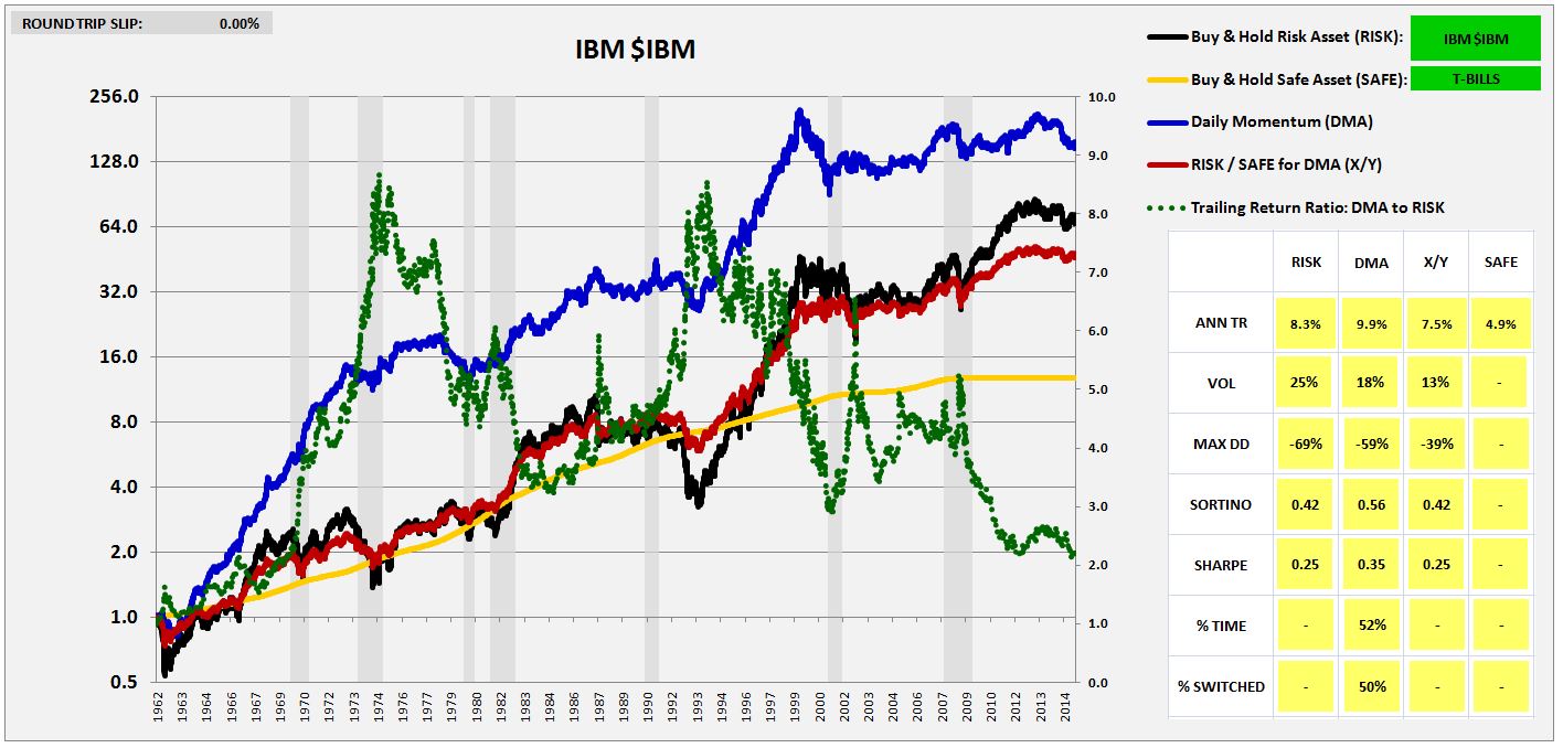
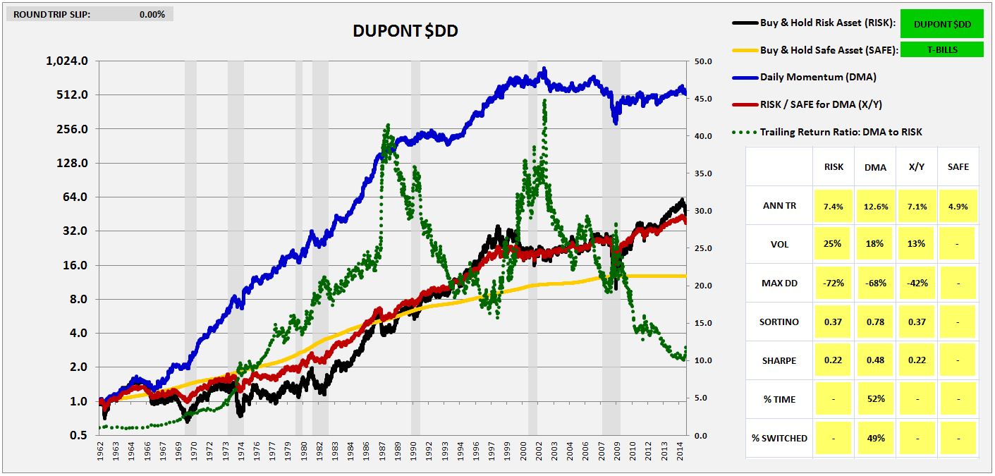
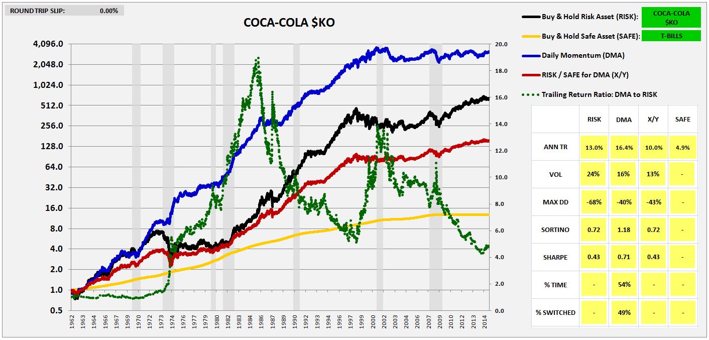
The following six charts show the results of backtests of the Daily Momentum strategy from 1963 to 2015 on the total U.S. market and on five well-known individual large cap names: Caterpillar $CAT, General Electric $GE, International Business Machines $IBM, Dupont $DD, and Coca-Cola $KO. All returns are total returns with dividends reinvested at market. To make any potential “stale price” effect maximally apparent, a 0% slip is used.
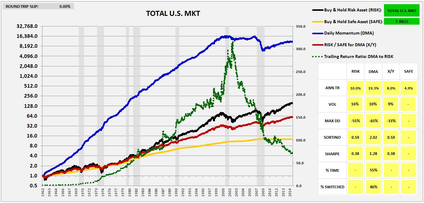
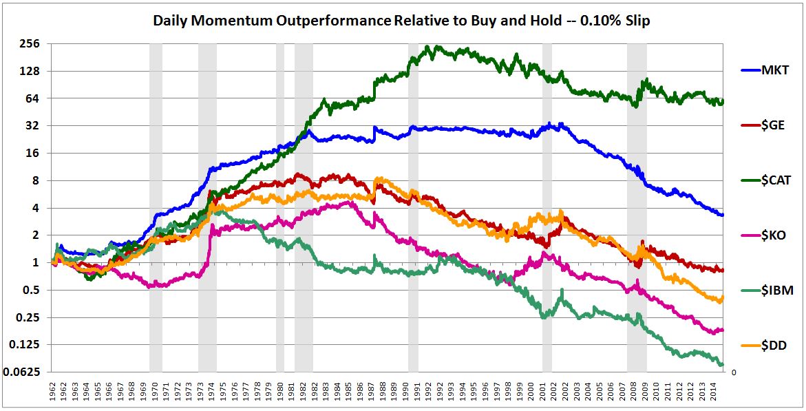
The following two charts show the outperformance of Daily Momentum relative to Buy and Hold (ratio between the two) on a log scale for each of the names and for the total market. The applied slip is 0% in the first chart and 0.10% in the second:
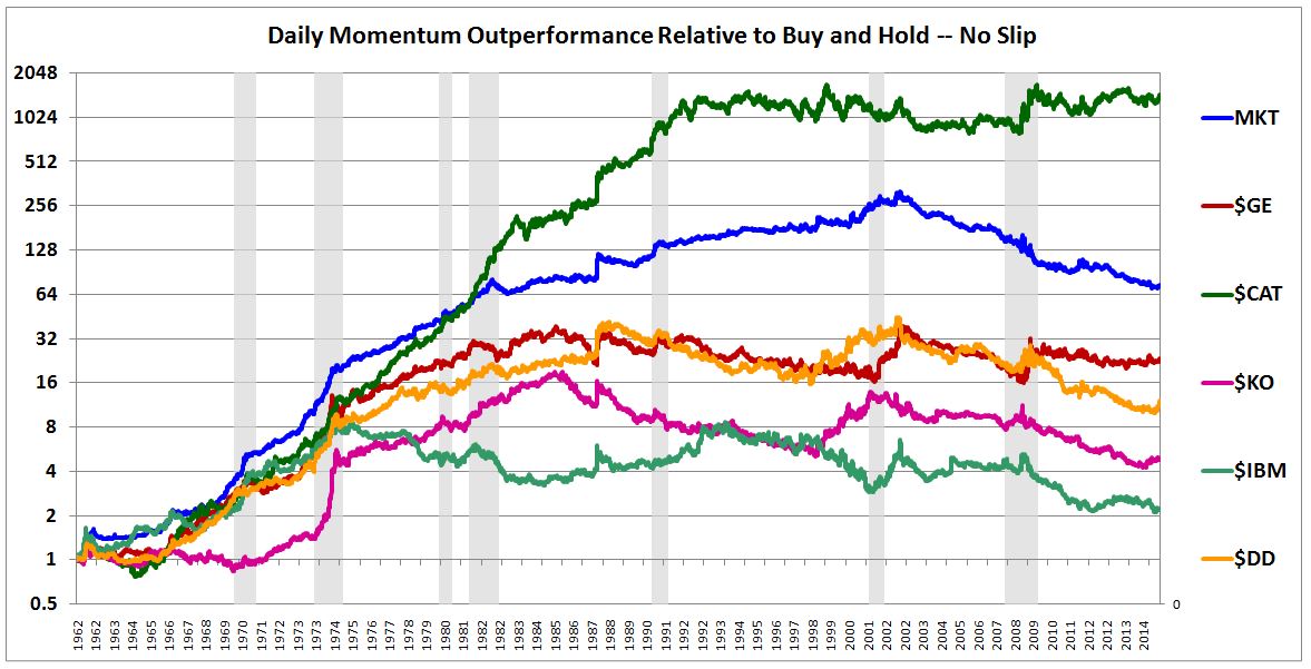
As you can see in the charts, the strategy continues to outperform in the early half of the period, so the “stale price” effect cannot be the entire story. At the same time, with the exception of Caterpillar, the strategy’s outperformance in the individual names is less pronounced than it is for the the index, which suggests that the “stale price” effect–or some other index-related quirk–is driving a portion of the strategy’s success in the index case.
Interestingly, the strategy’s outperformance died off at different times in different names. Using a 0% slip, the strategy’s outperformance died off in 1974 for IBM, in 1985 for GE and Coke, in 1988 for Dupont, in 1992 for Caterpillar, and in 2000 for the total market. This observation refutes the suggestion that the breakdown is uniquely related to something that happened in the market circa the year 2000, such as decimalization. In individual securities, the phenomenon had already disappeared decades earlier.
Concerns About Momentum
In the prior piece, I presented a chart of the outperformance relative to the overall market of each value-weighted decile of the Fama-French-Asness Momentum Factor from 1928 to 1999, and then from 2000 to 2015. The purpose of the chart was not so much to challenge the factor’s efficacy in the period, but simply to show the reasonable decay concern that caused me to look more closely at the performance of momentum after the year 2000, and that prompted me to stumble upon Daily Momentum, with it’s weird break around that date.
A number of readers have e-mailed in asking me to separate out the 1928 to 1999 chart into 15 year increments, to allow for an apples-to-apples comparison of the factor’s efficacy across all 15 year periods. Here, then, are the requested charts, in 15 year increments, from 1927 to 2015:
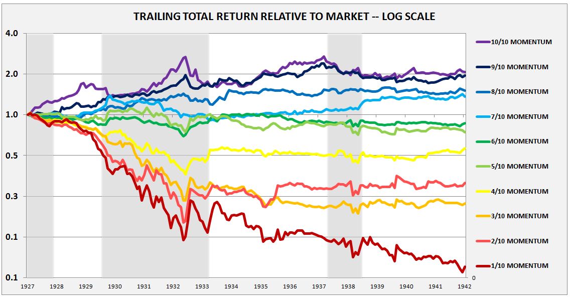
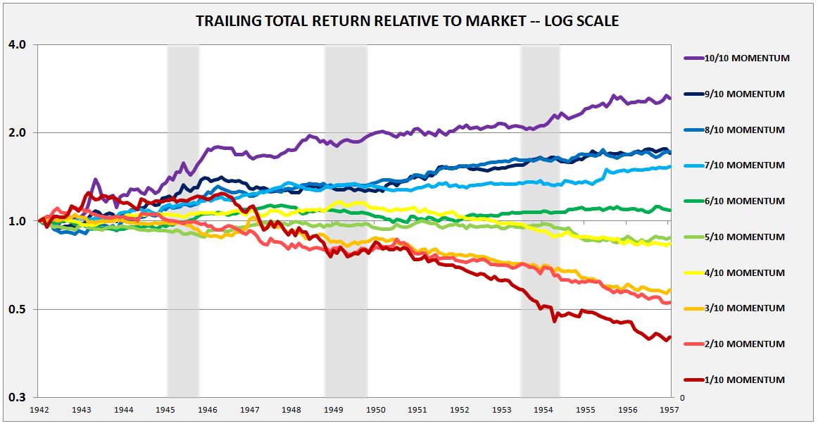
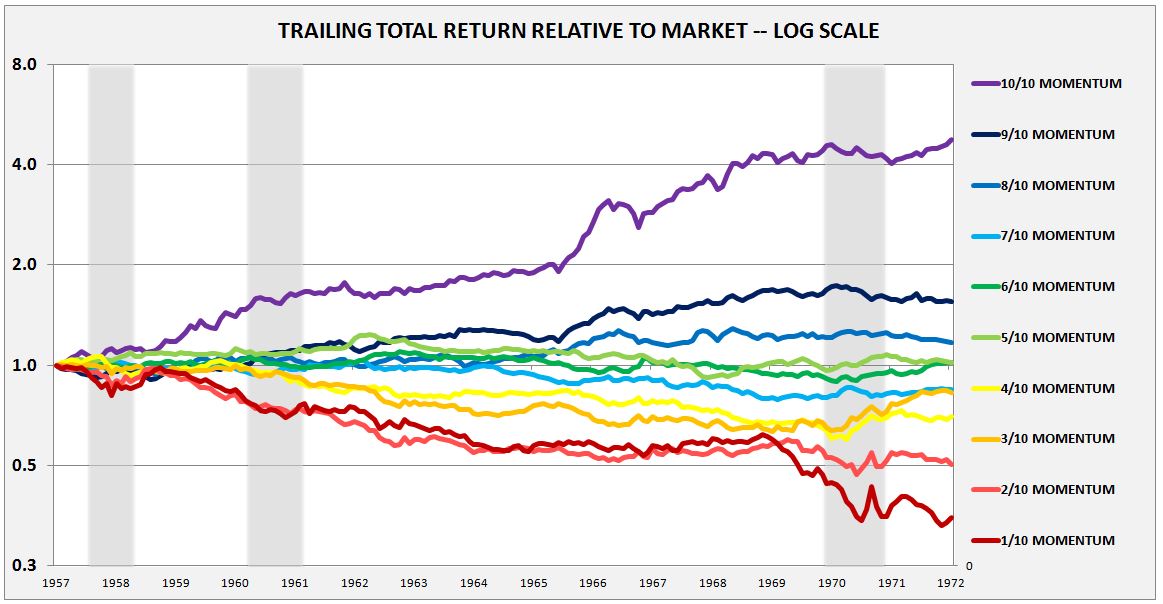
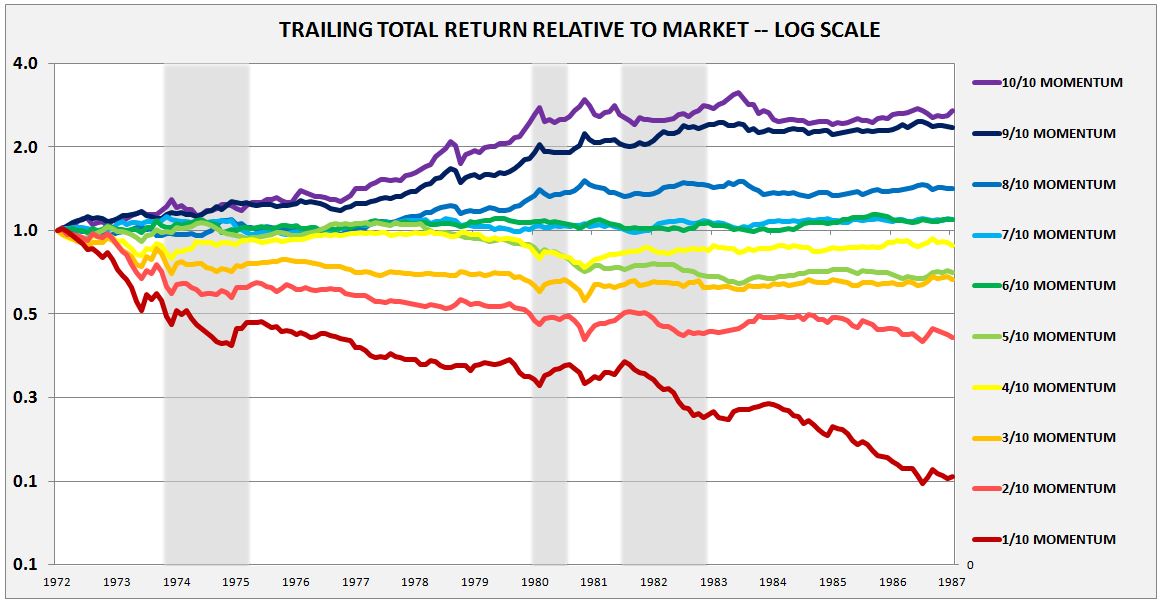
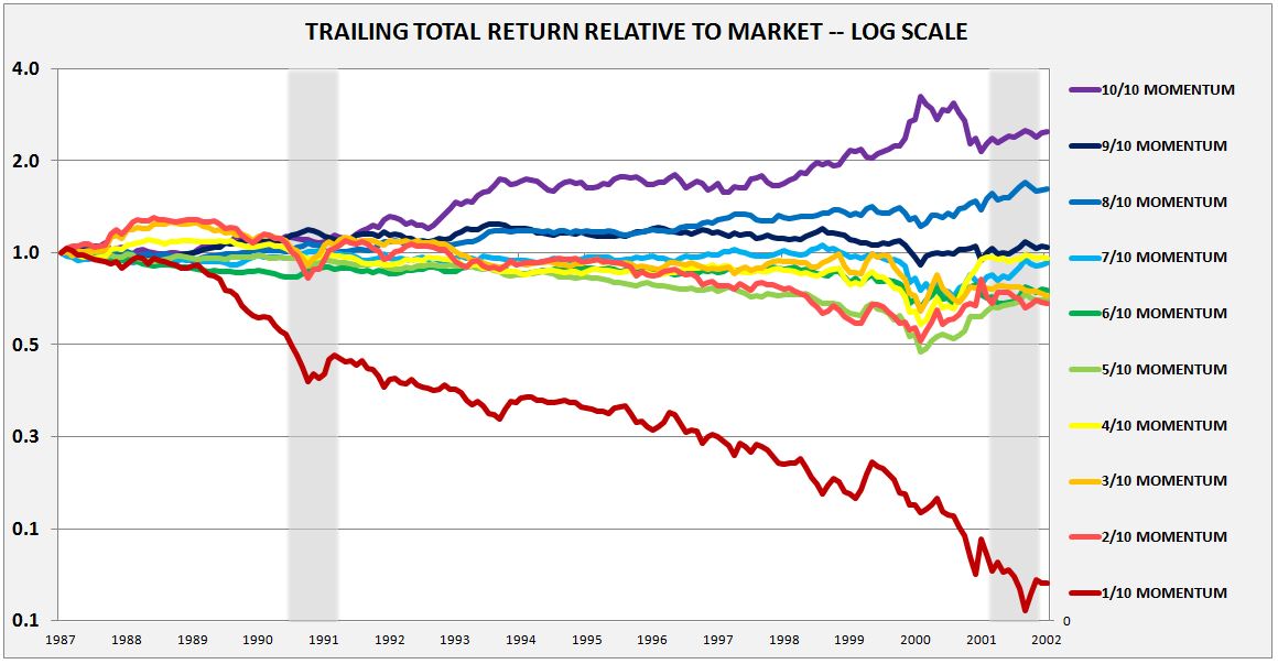
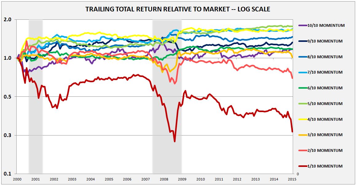
Clearly, when it comes to the performance rankings, the last chart is different from the others. Momentum still outperforms, but the outperformance isn’t as pronounced or as well-ordered as in prior periods.
The idea that the efficacy of momentum would decay over time shouldn’t come as a surprise. How could it not decay? For a strategy to retain outperformance, there have to be barriers to entry that prevent its widespread adoption. From 1928 to the early 1990s, momentum’s barrier to entry was a lack of knowledge. Nobody in the market, save for a few people, knew anything about the phenomenon. What is momentum’s barrier to entry today, when every business school student in the country learns about the phenomenon, and where any investor that wants to directly harvest its excess returns has 10 different low-cost momentum ETFs to choose from?
Some have suggested that the counter-intuitive nature of momentum, the difficulty that people have in understanding how it could be a good investment strategy, might serve as an effective barrier to entry. Maybe, but I’m skeptical. In my experience, investors–both retail and professional–are perfectly willing, and often quite eager, to invest in things that they do not fully understand, so long as those things are “working.”
It seems, then, that one of two things will likely end up happening: either momentum will not work like it used to, or it will work like it used to, and money will flock into it, either through the currently available funds, or through funds that will be set up to harvest it in the future, as it outperforms. The result will either be a saturation of the factor that attenuates its efficacy, or a self-supporting momentum bubble that eventually crashes and destroys everyone’s portfolio.
Ask yourself, as the multitude of new momentum vehicles that have been created in the last few years–for example, Ishares $MTUM, which now has over $1B in AUM and growing–accumulate performance histories that investors can check on Bloomberg and Morningstar, will it be possible for them to show investors the kinds of returns relative to the market seen in the purple line below, and not become the biggest funds on earth?
In my opinion, to avoid saturation and overcrowding, particularly in the increasingly commoditized investment world that we live in, it won’t be enough for momentum to be counter-intuitive. If a fund or a manager’s performance looks like the purple line above, people will not care what the mechanics were. They will simply invest, and be grateful that they had the opprtunity. Given that momentum’s counter-intuitiveness won’t work as a barrier, then, all that is going to be left is underperformance. The factor will need to experience bouts of meaningful underperformance relative to the market, underperformance sufficient to make investors suspect that the strategy has lost its efficacy. Then, investors will stay away. The problem, however, is that the strategy may actually have lost its efficacy–that may be the reason for the underperformance. Investors won’t know.
To be clear, when I talk about momentum underperforming, I’m not talking about the underperformance of a long-short momentum strategy. A long-short momentum strategy that rebalances monthly will experience severe momentum crashes during market downturns. Those crashes are caused by rebalancing into 100% short positions on extremely depressed low momentum segments of the market. When the market recovers, those segments, which represent the junk of the market, explode higher, retracing the extreme losses. The increase in the 100% long position during the upturn fails to come close to making up for the extreme rise of the 100% short position, which is rebalanced to a 100% position right at the low. The result ends up being a significant net loss for the overall portfolio during the period.
Instead, I’m talking about the underperformance of simple vanilla strategies that go long the high momentum segments of the market. As the charts show, those segments have almost always outperformed the index. Where they’ve underperformed, the underperformance hasn’t lasted very long. For them to underperform in a meaningful way–enough to make the performance uninspiring to investors–would be a significant departure from past performance.
What is momentum’s sensitivity to saturation and overcrowding? How much money would have to flow into the the factor to dampen or eliminate its efficacy, or worse, turn it into an underperformer? What amount of underperformance is needed to keep a sufficient number of investors out, so that the strategy can retain its efficacy? How much will this underperformance detract from momentum’s overall excess returns over the market? What is the mechanism of the underperformance? Is it a gradual decay, or a crash that occurs after a momentum bubble bursts? Is the right answer to try to time the underperformance–to exit momentum when it’s popular, and re-enter it when it’s out of favor? If so, what are the signs and signals? These are all important questions. Since there isn’t any relevant data to go off of–the first experiment on the subject is being conducted right now, on us–investors will have to answer the questions directly, working out the complicated chess position themselves, without the help of historical testing.