Global Stock Market Valuation and Historical Real Returns Image Gallery

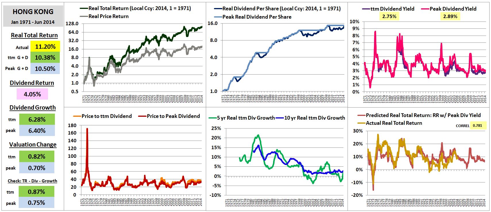
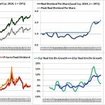
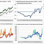
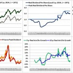
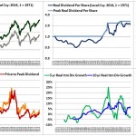
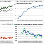
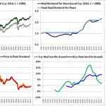
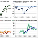
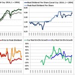
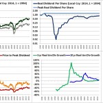
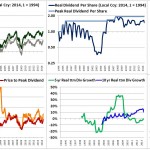
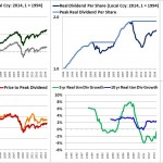
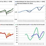
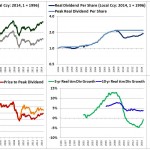
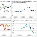
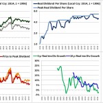
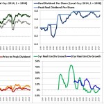
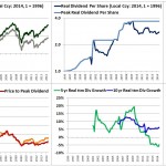
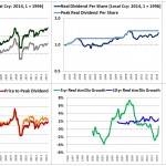
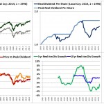
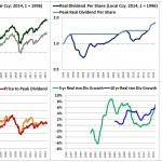
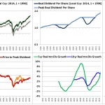
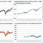
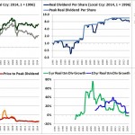
In this piece, I’m going to analyze the historical local currency real total returns of different stock markets around the world: 46 different large cap indices, 12 different small and mid (SMID) cap indices, and, for the U.S., 4 different style indices–growth, momentum, quality, and value.  For each index, I’m going to generate a chart that visually captures key trends and data points, shown below with the Hong Kong stock market as the example:

Theoretical background, and instructions for how to read and interpret the charts, are provided in the paragraphs below.  The charts are presented at the end.

Dividend Decomposition

We can decompose–separate, conceptually split apart–equity total returns into two components:

• Dividend Return: the return due to dividends paid out and reinvested.

• Price Return: the return due to changes in the market price

We can further decompose price return into two components:

• Growth: the return due to growth in some chosen fundamental

• Valuation: the return due to changes in market valuation measured in terms of that fundamental

To measure fundamental growth, we can choose any “fundamental” that we want, as long as the metric that we use to measure the change in valuation employs that same fundamental.  So, for example, we can decompose the price return into: the return due to earnings growth and the return due to the change in the price to earnings multiple.  Alternatively, we can decompose the price return into: the return due to book value growth and the return due to the change in the price to book multiple.  And so on.  We cannot, however, decompose the price return into: the return due to earnings growth and the return due to the change in the price to book multiple.  On such a decomposition, we would be mixing incompatible bases.

To conduct the decompositions, we’re going to use dividends as the fundamental.  We’re therefore going to decompose the real returns of each market into three components: the real return due to dividends paid out and reinvested at market prices, the real return due to growth of dividends, and the real return due to the change in the price to dividend multiple–which is just the inverse of the dividend yield.  Notice the aforementioned consistency between the fundamental and the valuation measure: we’re measuring fundamental growth in terms of dividend growth and changes in valuation in terms of changes in the price to dividend ratio.

We need to conduct the analysis in real terms–with each country’s returns adjusted for inflation–because inflationary growth is worthless to investors, yet it’s a significant driver of nominal equity returns–often, the most significant driver of all.  If we don’t adjust the returns for inflation, then the performance of the stock markets of high-inflation countries such as Hungary will appear vastly superior to the performance of the stock markets of low-inflation countries such as Germany, even though the performance is not any better in real terms.

There are three reasons why we’re going to use dividends as the fundamental, rather than earnings.  First, dividends are more stable across the business cycle than earnings.  Second, the accounting practices used to measure earnings are not the same across different countries, different periods of history, or even different phases of the business cycle.  But dividends are dividends–unambiguous, concrete, indisputable.   Third, for international markets, historical dividend data is more readily available than historical earnings data. MSCI provides total return and price return indices for all countries that have investible stock markets (available here).  In providing those indices, MSCI provides the materials necessary to back-calculate dividends across history.  We’re going to use the MSCI indices, which generally go back to 1971, along with international CPI data (available here), to conduct the decompositons.

Note that the dividends that we back-calculate in this way will be somewhat different from what you might see in an ETF or from an official indexing source–such as S&P or FTSE. As expected, the back-calculated dividends tend to closely match the dividend data on MSCI’s fact sheets, but even that data is not perfectly consistent with other sources.  Take any discrepancies lightly–it’s the big picture that we’re focused on here.

Now, the obvious problem with decomposing returns using dividends as the fundamental is that anytime the dividend payout ratio–the share of earnings that corporations pay out to their shareholders in the form of dividends–changes in a lasting, secular manner, we’re going to get distorted results.  Unfortunately, there’s no way to avoid this problem–we just have to deal with it.

Fortunately, most countries have maintained relatively consistent dividend payout ratios across history.  The U.S. is the obvious exception–but even with the U.S., the ensuing distortion isn’t too large, because in the historical period that we’re going to focus on–the early 1970s until the present day–dividend payout ratios haven’t changed by all that much.  The big downshift in payout ratios happened earlier, as you can see in the chart below, which shows smoothed dividends divided by smoothed earnings for the S&P 500:

Trailing Twelve Month Dividends and Peak Dividends

Like earnings, dividends are cyclical, though to a much lesser degree.  To smooth out their cyclicality, we’re going to conduct the price return decomposition using two different formulations of the dividend: first, the simple trailing twelve month (ttm) dividend, second, the peak dividend–the highest dividend paid out in any twelve month period at any time in the past.

The ttm dividend decomposition will separate the price return into ttm dividend growth and changes in the price to ttm dividend ratio. The peak dividend decomposition will separate the price return into peak dividend growth and changes in the price to peak dividend ratio.  Both decompositions will be presented in the charts so that the reader can compare them.

The best cases of hidden value are those where the ttm dividend yield is very low, but the peak dividend yield is very high.  A sharp divergence between the two suggests that the market is only taking into consideration the current dividend, which may be temporarily depressed, and is ignoring the past dividends that the corporate sector paid out–dividends that it may end up being able to pay out in the future, when the temporarily depressed conditions improve.

The chart to the left ranks the stock markets of the world in terms of peak dividend yield and ttm dividend yield as of June 30, 2014.  Looking at Greece in specific, on a simple ttm basis, the dividend yield at current prices is a paltry 2.41%–hardly a signal of value.  But if you look at the peak dividend yield, which uses the highest dividend in Greece’s history–the dividend paid in the ’06-’07 period–the dividend yield at current prices comes in at a whopping 23.35%.

Now, it may be the case that the performance that the Greek corporate sector exhibited in ’06-’07 does not accurately represent the performance it is likely to exhibit in the future, and that the long-term yield that Greece will offer at current prices will be significantly lower, even as conditions in  Greece improve.  But even if we assume that the long-term yield at current prices will be dramatically lower–say, 75% lower–that’s still a 6% yield, which is an excellent yield.

Familiar readers will note that the country’s that show up as cheap and expensive in terms of peak dividend yields also show up as cheap and expensive in Mebane Faber’s global CAPE analysis.  The two metrics are reasonably consistent in their signals, which is to be expected, given that they are reading the same valuation reality.  As a valuation metric, CAPE is admittedly superior to the peak dividend yield, but it’s also more costly–you have to use ten years to calculate it, which means that you lose 10 years from the analysis. For many of these countries–those that only have 20 or 30 years of history–10 years is a lot to lose.

The Goal of the Decomposition

So why are we doing this decomposition?  What’s the point?  The reason we do the decomposition is because it gives us a rough picture of how much of a given countries’ stock market performance has been driven by changes in valuation, and how much has been driven by fundamentals.  Changes in valuation are a fickle driver of long-term returns. If a country has outperformed because it has gone from cheap to expensive, or if it has underperformed because it has gone from expensive to cheap, then as investors we should want to go the other way–invest in the cheap country, and not invest in the expensive country.

But, crucially, if the country has outperformed because its corporate sector has exhibited consistently poor fundamental performance, then we don’t necessarily want to go the other way.  Warren Buffet reminds us that sound fundamental investing is not just about buying companies on the cheap, but about buying good companies on the cheap.  Bad companies on the cheap–value traps–are return killers.  This fact is just as true on the country level as it is on the individual stock level.

When we look at the data, we’re going to quickly notice that the corporate sectors of some countries have performed much better–produced substantially more fundamental growth for each unit of reinvestment that they’ve engaged in–than the corporate sectors of other countries.  This outperformance may have been the result of coincidental tailwinds that will not obtain going forward, and therefore extrapolating the outperformance into the future may prove to be a mistake.  But the outperformance may also be a sign of the inherent superiority of the corporate sectors of some countries relative to the corporate sectors of other countries.  If it is, then we should preferentially seek out the superior countries, and be willing to pay more to invest in them, and avoid the inferior countries, demand more to invest in them.  Valuation matters to returns, but it’s not the only thing that matters.

Countries with corporate sectors that invest inefficiently and excessively, and that don’t respect the rights and interests of their shareholders, don’t tend to produce strong returns, even when they are bought on the cheap.  Take the example of Russia–a country notorious for its corruption, corporate waste, poor governance, and disrespect for property rights. Since 1996, the Russian stock market has averaged an atrocious -5% annual real total return.  This disastrous performance was not the result of a high starting valuation–the dividend yield in 1996 was above 2%, higher than for the U.S.  Rather, the underpformance is a result of the fact that dividends haven’t grown by a single ruble in real terms since 1996, even though Russia hasn’t paid out very much in dividends along the way.  If the Russian corporate sector was earning profit and reinvesting that profit the entire time–a full 18 years–where did the profit go?  It certainly didn’t go to shareholders, as they have nothing to show for it.

On the other extreme, since 1996, the U.S. stock market has averaged a healthy 6% real total return.  This 6% has not been driven by any kind of irresponsible valuation expansion–in dividend terms, valuations were roughly the same in 1996 as they are today. Rather, it was the result of solid corporate performance.  The U.S. corporate sector produced a 2% annual real return from dividends paid out to shareholders, and an impressive 3.25% in annual real dividend growth.  Changes in the U.S. market’s valuation added an additional 0.75% annually to the real return, producing a real total return of 6%.

The Payout Ratio: Inevitable Messiness

Now, the picture we will get from the decomposition will be admittedly messy, for a number of reasons.  First, we aren’t incorporating the average dividend payout ratios of each country into the analysis, therefore we can’t assess the price to dividend ratio as a valuation signal.  Is a price to dividend ratio of 50–i.e., a dividend yield of 2%–high, and therefore expensive?  It may be for Austria, but not necessarily for Japan.  Not knowing the dividend payout ratio, all we can do is compare the country’s current valuation to its own history, on the assumption that dividend payout ratios haven’t changed in a long-term, secular manner (and, to be fair, they may have).

Moreover, because we don’t know the dividend payout ratio, we don’t know how much growth we should expect out of each country. Countries that are reinvesting a large share of their cash flows in lieu of paying out dividends should be producing large amounts of growth–those that are doing the opposite should not be.   Using the information currently available, we can’t necessarily tell the difference.

Most importantly, we don’t know what the factors are that have caused the corporate sectors of some countries to perform substantially better than others.  The factors could be cyclical, macroeconomic, demographic, era-specific, driven by differences in industry concentrations, investment efficiency, corporate governance, shareholder friendliness, unsustainable booms in productivity, and so on–we don’t know.  Therefore we can’t necessarily be confident in projecting the past superior performance out into the future.

Still, the picture we get will give us a minimally sufficient look at what’s going on.  It will tell us where things have been going well for shareholders in terms of the growth and dividends that have been produced for them, and where things have not been going well. That knowledge should be enough to get us started on the important task of figuring out where the corporate overachievers and the value traps might lie.

How to Interpret the Charts

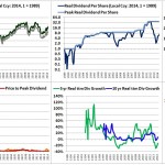
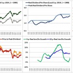
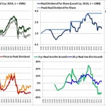
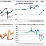
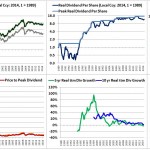
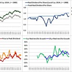
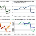
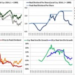
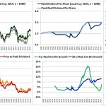
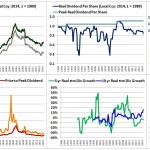
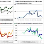
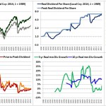
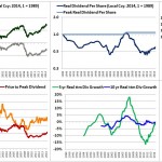
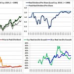
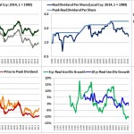
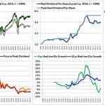
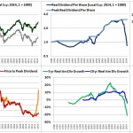
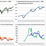
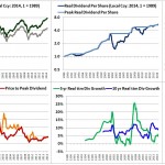
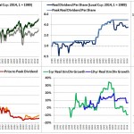
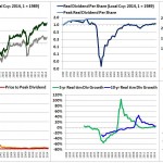
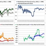
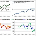
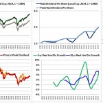
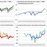
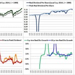
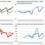
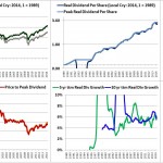
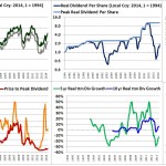
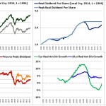
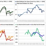
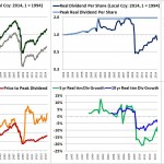
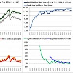
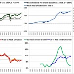
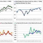
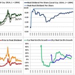
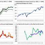
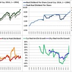
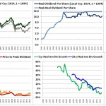
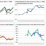
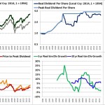
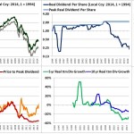
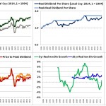
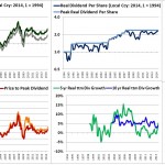
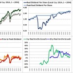
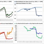
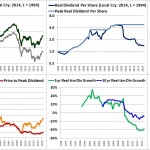
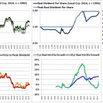
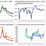
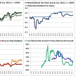
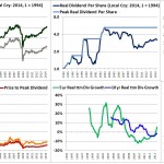
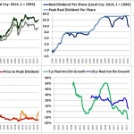
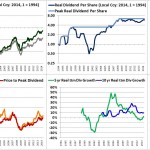
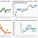
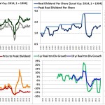
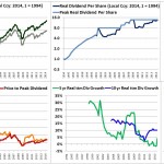
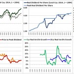
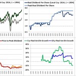
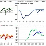
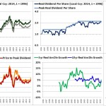
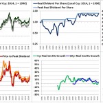
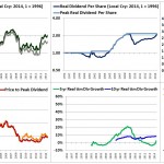
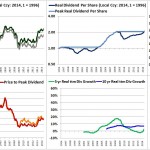
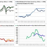
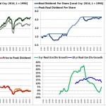
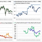
Consider the following chart, which decomposes the performance of Ireland from January 1989 to June of 2014:

The bright yellow in the left column (0.17%) is the actual annual real total return for the period.  The green (-0.68%) and blue (5.90%) below that is the annual real return contribution from growth plus dividends–which, notice, is what the real return would have been if there had been no change in valuation (the third component of returns removed).  The green (-0.68%) uses a ttm dividend basis, and the blue (5.90%) uses a peak dividend basis.

The pink below that (2.36%) is the annual contribution to real returns from reinvested dividends over the period.  It is calculated by taking the difference between the annual real total return for the period and the annual real price return for the period.  Below that is the annual contribution of dividend growth (-3.02%, 3.75%) and change in valuation (0.85%, -5.73%), measured under each basis (green = ttm dividend basis, blue = peak dividend basis).  Below that is an internal checksum of sorts, in which the contribution of the valuation change is calculated by a wholely different method, to make sure that the analysis is roughly correct.  You can ignore it.

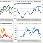
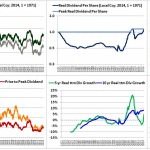
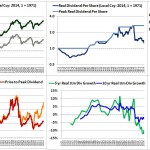
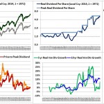
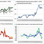
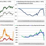
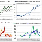
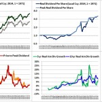
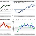
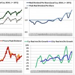
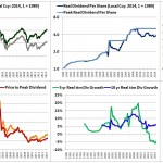
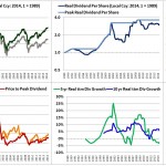
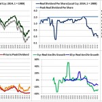
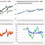
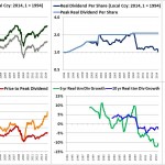
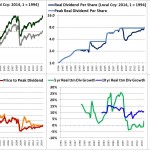
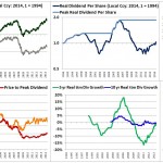
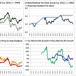
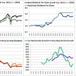
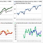
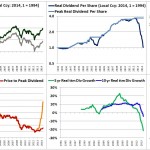
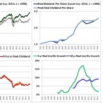
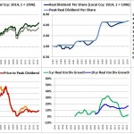
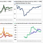
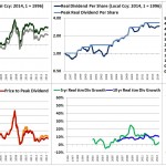
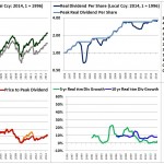
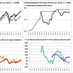
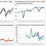
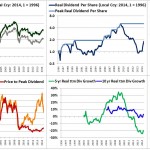
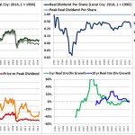
In terms of the graphs, the upper left graph is the real total return (green) and the real price return (gray).  The upper middle graph is ttm real dividends per share (dark blue) and historical peak real dividends per share (light blue).  The upper right graph is the historical yield using the ttm dividend (purple, with the yellow box above showing the ttm dividend yield as of June 2014, which is 1.67%) and the peak dividend (hot pink, with the yellow box abvoe showing the peak dividend yield as of June 2014, which is 9.26%).  To review, the peak dividend yield is what the yield would be at a given time if the dividend went back to what it was at the largest point in time up to that time–for Ireland, it’s very high, because the dividends that Ireland paid out in the last cycle were very high relative to Ireland’s current price, which is depressed–you can interpret this as a sign of cheapness for the Irish market).  The lower left graph is the Price to ttm Dividend ratio (orange) and Price to Peak Dividend ratio (red) ratio.  The lower middle graph is the 5 year (light green) and 10 year (bright blue) growth rates of the real ttm dividend.

The lower right graph is a running estimate of future 5, 7, and 10 year Shillerized real returns using the “real reversion” method laid out in a prior piece.  We calculate this estimate by discounting the market’s average real return to reflect a reversion from the present valuation to the average valuation.

Now, let me be fully up front with the reader.  Like all backward-looking return estimates that purport to fit with actual forward-looking results across history, this estimate involves cheating.  We are using information about the average return for the entire data set, past and future, and the average valuation for the entire data set, past and future, to estimate the future return from past moments in time.  From the perspective of those moments, the average of the entire data set includes information about the future that was not known then–therefore, in projecting a reversion to the average, our estimates are taking a peak at the future.  That is, they are cheating.

You’ll see that the method often nails it, with extremely high correlations with actual returns, well above 90%. But don’t take that to mean anything special. As I’ve emphasized elsewhere, these types of fits are very easy to build in hindsight, because you can effectively peak ahead at the actual results, and utilize now-determined information about the future that was not determined–or knowable in any way–at the time that the prediction would have needed to have been made.

I introduce the real reversion estimates into the chart not to make any sort of confident prediction about what the forward real return of any given market will actually be–such a prediction would require a look that goes much deeper than a backwards-looking curve fit that exploits cheating–but simply to give the reader an idea of when, in the market’s history, valuations were cheap and expensive relative to their averages for the period, and where they are now, relative to their historical averages.  The averages for the period in question may not end up being the averages of the future, and therefore they may not be relevant to the future.

The Charts With Associated Tables

Finally, to the charts.  What follows is a user-controlled slideshow of charts for different countries across different time periods of history.  If you click on any image, it will put you into that country’s part of the slideshow.

Before each chart, there’s a table, sorted by country name, that presents all of the results.  To view the table, simply click on it.  On the right side of each table, there’s a section on “non-equity growth”, which includes potentially relevant information on population growth, real GDP growth per capita, and real GDP growth over the period (source here).

Jan 1971 to Jun 2014: Developed Market Returns

Table:

Slideshow:

Jan 1989 to Jun 2014: Developed and Emerging Market Returns

Table:

Slideshow:

Jan 1989 to Jun 2014: US Growth, Momentum, Value, Quality

Table:

 

Slideshow:

Jan 1994 to Jun 2014: Developed, Emerging and Frontier Market Returns

Table:

Slideshow:

Jan 1996 to Jun 2014: Developed and Emerging Market Small and Mid Caps

Table:

Slideshow:

1996 to 2014: Czech Republic, Egypt, Hungary, Russia

Table:

Slideshow:

Conclusion

After examining the data, here are my conclusions:

• Europe, in particular the PIIGS, are very cheap relative to their own valuation histories and relative to the valuations of other countries.  On a ttm dividend basis, the returns due to growth have been poor, but that’s because dividends have crashed to almost nothing in response to the crisis.  If dividends eventually return to where they were prior to 2008–a big if, but one worth considering–the returns of the European periphery countries, and of European countries in general, should be very attractive.

• Japan’s underperformance since 1989 has been due primarily to an egregiously high starting valuation.  But this excess has been entirely worked off, and Japan now offers a higher dividend yield than the U.S.  Japan’s corporate performance, however, remains something of a mystery.  It’s hard to quantify Japan’s dividend payout ratio, and to therefore get an estimate of how much dividend growth should have occurred from 1989 to today, because Japanese earnings are significantly understated due to excessive depreciation.  If the Japanese dividend payout ratio relative to true earnings has been low, which it probably has been, then Japanese ROEs have been poor.  The country owes its shareholders more growth for the amount that it has allegedly “reinvested.”  If growth by capital investment is not possible in Japan given the aging, shrinking population demographics, and weak consumer demand, then earnings should be deployed into dividends and share buybacks.  If Abenomics manages to stimulate this outcome, and promote an associated improvement in shareholder yield, then Japanese equities should produce strong returns going forward.

• Australia and New Zealand are reasonably valued, with healthy dividend yields.  But the commodity-centric earnings and dividends that they generated in the last cycle may not be sustained going forward.

• The US is expensive relative to its own history and relative to other countries.  It’s among the most expensive stock markets in the world.

• Emerging Markets are generally cheap, but, macroeconomically, it’s difficult to project their performance over the last 20 to 30 years out into the future.  Interesting countries to look at on valuation include Brazil, Singapore, and Taiwan.  Korea and Turkey, in contrast, are hardly cheap on a dividend basis, and have not performed well in terms of the amount of dividend growth that they have generated.

• Russia and China are, at a minimum, weird.  Both have exhibited extremely volatile markets over the last 18 years, with dividend fluctuations tracking the price fluctuations.  Russia, in particular, has generated no real dividend growth since 1996, and also no real dividend growth since 2003, after the default.  Both markets are presently very cheap, but they won’t make for good investments unless they cease to be the value traps that they’ve proven themselves to be in the past.

• For styles, counterintuitively, the “value” sector of the U.S. market is expensive, and the “quality” sector is cheap.  So if you’re looking to invest in the U.S., you’re best bet is probably to buy high quality multinationals with strong competitive moats–the kind that Jeremy Grantham of GMO frequently touts.

• For small and mid caps, the US and the UK, though unquestionably expensive, may not be as egregiously expensive as some seem to think.  Their dividends are basically at the historical average since 1996.  Singaporean and Canadian small and mid caps, in contrast, appear very attractively valued.

• The Nordic countries–Sweden, Norway, Finland, and Denmark–have produced fantastic dividend growth for their shareholders, on pretty much all measured horizons.  With the exception of Denmark, these countries are all reasonably valued at present–but, of course, we can’t be sure if the stellar dividend growth will continue.

• It’s difficult to find a connection between macroeconomic aggregates–population growth, GDP per capita growth, and GDP growth–and returns.  If anything, we can probably say that healthy, moderate, positive population growth, with moderate GDP per capita and GDP growth, are better for returns than the opposite.