Using Total Return EPS to Decompose Historical S&P 500 Performance: Charts from 1871 to 2015

In this piece, I’m going to do five things:

• First, I’m going to clarify the purpose of Total Return EPS, what it’s trying to accomplish.  In a single sentence, the purpose of Total Return EPS is to convert dividends into EPS so that the fundamental sources of return can be added together into one single term whose past growth rate can be analyzed and whose likely future growth rate can be projected.

• Second, I’m going to explain why the trend growth rate of Total Return EPS for the S&P 500 (~6%) is roughly equal to the historical average return on equity for the U.S. corporate sector (~6%).  The explanation will include a proposed theory for why return on equity generally reverts to the mean, and also for why it may not revert to its prior mean in the present environment.

• Third, I’m going to address a question that a significant number of readers have asked: why does Total Return EPS assume that buybacks occur at fair value, rather than at market prices?

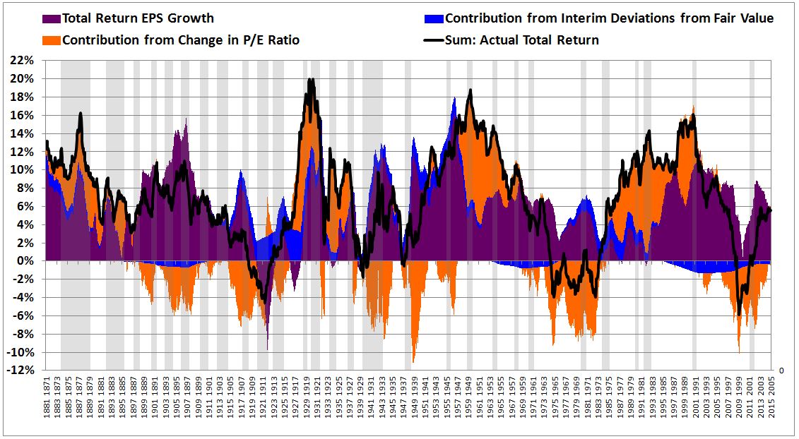
• Fourth, I’m going to show how actual total return can be “decomposed”–i.e., separated out–into three contributing components: (1) Total Return EPS growth, which consists of regular EPS growth plus the return from reinvested dividends (or hypothetical share buybacks), (2) the return contribution from the change in valuation–in this case, the change that occurs in the ttm P/E ratio from price to sale, and (3) the return contribution from interim deviations from fair value–a neglected source of return that arises from the valuations at which dividends are reinvested (or at which shares are hypothetically repurchased), and therefore the rate at which they accrete.

• Fifth, I’m going to present charts of these components for the S&P 500 from 1871 to 2015, on time horizons of 10, 20, 30, 40, 50, 60, and 70 years.

Three Options: Dividends, Expansion, Repurchases

When the corporate sector earns profit, it can do one of two things: distribute the profit to shareholders as dividends, or reinvest the profit.

• When it distributes the profit to shareholders as dividends, the shareholders get a direct return–a direct deposit of money into their accounts.

• When it reinvests the profit, the shareholders get an indirect return–“growth.” The profits earned in future periods, and the future dividends that can be paid from them, increase in size.  In an efficient market, this increase coincides with an increase in the market prices of shares, allowing shareholders to realize a return by selling.

Looking closer at the second option, the corporate sector can reinvest profit in one of two ways: by using it to fund business expansion, or by using it to repurchase equity (or debt). Both options produce growth in earnings per share (EPS).

• When the corporate sector uses profit to fund business expansion, it adds new capital that it can use to produce and sell additional output to the economy, from which additional income can be earned.  It grows the EPS by growing the E.

• When the corporate sector uses profit to repurchase equity–for example, by buying back shares on the open market and then cancelling them–it grows the EPS by shrinking the S.  (Note: The corporate sector can also use profit to repurchase or retire debt.  We can view this option as roughly equivalent to the repurchase of equity. Both options entail a reduction in the number of outstanding claims on the corporate sector, rather than an increase in the size of the corporate sector’s operations).

What we have, then, are three destinations for corporate profit: (1) the payment of dividends, (2) investment in business expansion, and (3) the repurchase of equity (or debt).  The first option entails a direct return, a direct deposit of money into shareholder pockets.  The second and third options entail an indirect return, achieved through growth in EPS.

EPS Growth: In Search of a Trend

What we want to know is the “trend” (or “normal”) rate of growth of EPS.  Knowing that trend rate would allow us to roughly estimate the likely future trajectory of EPS, given its position relative to trend.

To illustrate, suppose that the trend rate of EPS growth is 4% per year, but that EPS over the last several years hasn’t grown at all, or worse, has fallen substantially.  We would then expect future EPS growth to be higher than the trend rate, higher than 4%, as EPS catches up.  We would expect there to have been some kind of stunting process–say, a depression in profit margins–that explains the underperformance relative to trend, and that entails the potential for future outperformance, to be unleashed in an eventual mean-reversion.

The problem, of course, is that when we look at the historical data, we do not find a stable, reliable trend growth rate in EPS.  Instead, we find a trend growth rate that has increased substantially over time.  The following table shows averages of rolling 10 year annualized real EPS growth rates for the S&P 500 for the periods 1871 to 1930, 1930 to 1990, and 1990 to 2015, with each period beginning and ending in January:

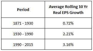
As  you can see in the table, the average rolling growth rate seen from 1990 to 2015 is four times the rate seen 100 years before it.  And note that this rate is the growth rate of GAAP EPS.  It include the effects of the questionable accounting writedowns that took place in 2003 and 2009.  If we use a corrected version of EPS that excludes those writedowns, the rolling average growth rate for the period increases to 4.76%–more than six times the rate achieved 100 years before it.

The reason for the increase in the trend growth rate of EPS is no mystery.  EPS growth varies inversely with the share of profit that is paid out as dividends.  That share has fallen over time.  The following table shows average payout ratios for the periods in question:

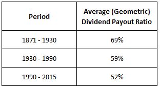
Now, there’s a legitimate question to ask here.  How much EPS growth should a given reduction in the dividend payout ratio actually produce? Is the observed increase in the growth rate, from 0.72% to 3.16%, commensurate with the observed decrease in the average payout ratio, from 69% to 52%?  Sadly, there’s no way to know.  Because we have no way to know, we can’t be sure that the reduced payout ratio is the only factor, or even the main factor, driving the increased growth.  For all we know, there could be some other factor driving it, a factor that will substantially impact growth going forward, either positively or negatively.

Return on Equity and Fundamental Total Return

We can distinguish between two sources of shareholder total return.  The first source is “fundamental”, and arises from the payment of dividends and the growth of EPS (or some other relevant fundamental).  The second source is “nonfundamental”, and arises from changes that occur in the valuations of assets between the time of purchase and the time of sale.  If you buy an asset and it pays you a dividend, or its price goes up in response to growth in relevant fundamentals–sales, earnings, net asset values, and so on–that is a “fundamental” return.  If you buy an asset and its price goes up independently of any type of growth in fundamentals–somebody just offers to pay you a higher price for the asset, because they want it more than the next person–that is a “nonfundamental” return.

The item that follows a consistent trend over time is not EPS growth per se, but the fundamental total return that accrues to shareholders–the return that dividends and EPS growth combine to produce.  Let me now explain why that return follows a consistent trend.  Bear with me.

The fundamental total return that accrues to shareholders is a function of the return that corporations generate on their equity, on the amount of capital that was invested to form them.  That return, after all, has to go to someone; it goes to the shareholders, those that made the investment, that put the capital in.

Now, return on equity (ROE) is mean-reverting.  When ROE is high in a given sector or industry, new investment flocks in, seeking to capture the high return.  The new investment leads to excess capacity, increased competition, weakened pricing power, and a reduction in profit that pulls the ROE for the sector or industry back down. When ROE is low in a given sector or industry, new investment stops happening.  The reduction in investment leads to an eventual undercapacity, reduced competition, increased pricing power for the remaining firms, and an increase in profit that pushes the ROE for the sector or industry back up–assuming, of course, that the goods and services being produced are actually wanted by the economy.  If they are not wanted, then the ROE for the industry or sector will go to zero, which is where it belongs for those that make unwanted things.

We’re currently seeing a textbook case of this process play out in the energy sector.  The economy needs a certain amount of oil.  The prior market price of oil–$75+–reflected the marginal cost of producing that amount, plus the extra “oomph” that speculation probably added.  But then efficient new drilling techniques were developed.  The strong profits that these techniques could earn with oil at $75+ led to an investment boom.  The investment boom eventually created an overcapacity that has pushed the price of oil down and that has dramatically lowered the return.  New investment has therefore dried up–and will stay dried up–until an undercapacity develops that increases the price enough to make the return attractive again.

This process of mean-reversion functions at its fiercest in the energy sector, where the good being sold is a pure commodity, and where there are few barriers or “moats” to block out competition and new entry.  But it applies in a general sense to all sectors and industries, and to the aggregate corporate sector as well.

(Caveat: If an economy evolves in a way that entails an increase in the number of barriers and “moats” in place to block out competition and new entry–i.e., in a way that makes it harder for new capital to partake in the high returns that existing capital might be enjoying–then the “mean” that the return on equity reverts to might increase accordingly. It remains an open question as to whether the new technology economy, with its tendency to produce winner-take-all scenarios in which the first mover is forever protected from competition–think $MSFT, $FB, $GOOG, $AAPL, and so on–has provoked such an increase.  I suspect that there is at least some of that effect at play in the much-discussed increase in ROEs and profit margins that we’ve seen take place over the last 20 years.)

Now, because the fundamental total return to shareholders is a function of the ROE, and because the ROE is mean-reverting, the fundamental total return to shareholders–paid out to them in dividends and growth–is similarly mean-reverting. Its mean-reverting nature is the reason that it follows a reliable trend over time.

Some might find this point hard to grasp–it’s admittedly hard to explain. To get a better feel for it, just think about the fundamental return that accrues to energy sector shareholders–shareholders in companies like $XOM and $CVX.  Can you see how the process that produces mean-reversion in energy sector ROEs would also produce mean-reversion in the fundamental return that $XOM and $CVX shareholders receive over time?  The same operating environment that allowed those companies to generate outsized fundamental returns–outsized EPS growth and outsized dividends–when oil was $75+ is what pulled in all of the new investment that fueled the current overcapacity, the squeeze to find buyers of all of the output, that is now pushing those same fundamental returns back down, hedges notwithstanding.

If there had been no new oil to drill, then that would have been a very powerful “moat”, and the high returns that these companies enjoyed might have been sustainable.  But when there is a new discovery that opens up ample new supply with the promise of a high return to anyone with capital that wants to make an investment in it, the high returns–to the new entrants and the existing players–simply will not last.

Ideally, then, we would ditch the effort to find the trend growth rate in EPS, and would instead focus on finding the trend in the metric that actually follows a trend–fundamental total return.  The problem, of course, is that fundamental total return is tied up in two distinct types of terms: EPS growth and dividends.  To properly analyze the trend in that return over time, we need a way to convert the terms into the same type of term, so that they can be added together to produce a single term, a single index.

The optimal way to solve the problem is to convert the dividends into a type of additional EPS, and then add the additional EPS to the actual EPS.  Then, we will end up with one single term that grows over time at a consistent trend rate, whose position relative to trend we can examine and make informed future projections based on.

That is precisely what the technique in the prior piece tries to do.  It tries to convert dividends into additional EPS by hypothetically assuming that dividends are diverted into share buybacks.  It then adds the additional EPS from the hypothetical share buybacks to the EPS that actually occurred, so as to form the unified, all-in-one term being sought: Total Return EPS.

The Equivalence of Reinvested Dividends and Share Buybacks

Now, from a total return perspective, it doesn’t matter whether a corporation chooses to distribute its profit as dividends, or use its profit to buy back shares.

• If it pays out dividends, the dividends will be reinvested (that’s at least the assumption that “total return” indices hypothetically make).  The reinvestments will cause the number of shares that each shareholder owns to grow.

• If it buys back shares, its outstanding share count will shrink, and therefore its earnings per share (EPS) will grow.  Mathematically, the growth in its EPS will roughly equal the growth in the number of shares that the shareholder would have come to own via dividend reinvestment.  If the market is efficient–meaning that it properly prices value–then the shareholder will end up no better or worse off, at least on a pre-tax basis (after tax, of course, is a different story).

Another way to express the point: When a corporation buys back shares with money that would otherwise have gone to dividends, it is effectively doing the dividend reinvestments for the shareholders.  It is accumulating shares in their names, as opposed to paying money out to them for them to accumulate shares on their own, independently of the company.  In truth, the two are not perfectly equivalent–share buybacks are actually slightly more accretive than reinvested dividends, for mathematical reasons that are too tedious to try to explain.  But they are close enough.

For any equity market, then, we are free to interchange dividends and share buybacks at will.  We can rebuild total return indices on the assumption that all dividends are hypothetically replaced with share buybacks, or that all share buybacks are hypothetically replaced with dividends–the replacements, if properly constructed, will have no perceptible effect on the total return.

The technique used to build the Total Return EPS index exploits this convenient equivalence.  It assumes, hypothetically, that for all of history, all dividend money that actually got paid was not actually paid, and was instead used to buy back shares.

When we examine Total Return EPS over history, we find that it does follow a reliable trend, as theory would suggest.  Consider the following table, which shows average rolling 10 year EPS and Total Return EPS growth rates over the periods identified in the previous table.

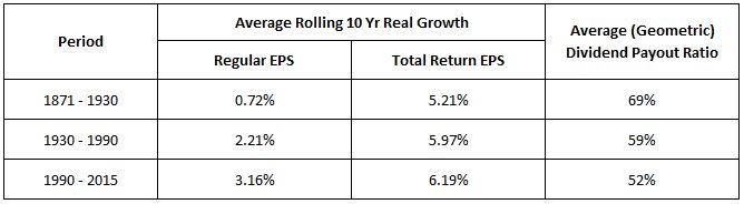
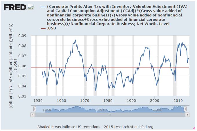
With Total Return EPS, we see a far more consistent growth rate.  That growth rate is roughly on par with the corporate sector’s average historical return on equity, some number close to 6%, as theory would again suggest (FRED).

Buybacks: Why Fair Value Prices?

The hypothetical buybacks that are used to form the Total Return EPS are assumed to occur not at market prices, but at fair value prices–prices that correspond to an average valuation across history.  A number of readers have tweeted and e-mailed in, asking why we make this assumption.  Why not assume that the buybacks occur at market prices instead, and save the confusion?

The reason is simple.  We’re trying to build an index that captures the fundamental total return that corporations generate for their shareholders through the profits they earn, which they deliver to their shareholders in the form of dividends and EPS growth.  If we were to conduct the buybacks at market prices, then that return would fluctuate based on the market’s valuation–a nonfundamental factor that has nothing to do with those profits.

In conducting the hypothetical buybacks, we are effectively converting dividends into a type of EPS (that gets added to the regular EPS to form the Total Return EPS).  That is, instead of paying out the dividends, we are using them to shrink the S, which effectively adds more EPS (makes EPS bigger by reducing the denominator).

Now, the valuations at which the buybacks occur represents the effective rate of conversion between dividends and EPS.  A low buyback valuation will convert dividends into a large amount of EPS, as the dividends will buy back a large number of shares. Conversely, a high buyback valuation will convert dividends into a small amount of additional EPS, as the dividends will buy back only a small number of shares.

To capture the true fundamental total return, and not add nonfundamental noise associated with where market prices just so happen to be, we need to ensure that the same rate of conversion between dividends and EPS is applied in all periods.  We need to ensure that each dividend, adjusted for size, adds the same amount of relative EPS as every other, regardless of when it happens to be paid.  That’s why we assume that all buybacks occur at the same valuation: “fair value”, which in the previous piece, we defined in terms of the historical average of the Shiller CAPE).

The assumption that the buybacks that underlie Total Return EPS occur at fair value may seem trivial and unimportant, but it makes a meaningful difference.  This difference will become particularly significant when we try to use Total Return EPS to build a new-and-improved Shiller CAPE.  If we use market valuations for the buybacks in Total Return EPS, the new-and-improved Shiller CAPE will end up skewed, giving an unnecessarily inaccurate picture of the market’s true valuation.  I plan to discuss the point in more detail in a later piece on the Shiller CAPE.

An Important Clarification: The Buybacks are Hypothetical

Let me now make an important clarification, based on some of the questions I’ve received. Regular S&P 500 EPS has continually grown throughout history.  Its growth has been driven by both business expansion (real economic investment that adds capital and increases output–EPS growth driven by growth in the E) and the repurchase of equity (buybacks, acquisitions, mergers, and so on–EPS growth achieved by shrinkage of the S).

The Total Return EPS doesn’t modify any of that growth.  Rather, what Total Return EPS does is add the additional growth that would have been produced if the dividends that were paid out had instead been used, completely hypothetically, to buy back shares (or fund acquisitions, mergers, and so on).

The following schematic makes the point more clear:

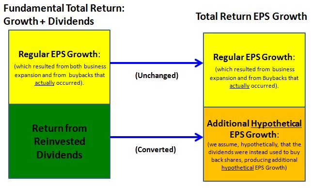
Some readers have asked: in constructing Total Return EPS, why do you assume that the buybacks occur at fair value prices, when, in reality, corporations like Apple and IBM are buying back their shares at market prices?   This question misses the point.  When I talk about conducting buybacks at fair value prices, I’m not referring to those buybacks, the ones that actually happened in reality, or that are happening now.  Their effects have already shown up, or will show up, in regular EPS growth.  The buybacks that I’m referring to, the ones associated with the construction of Total Return EPS, are hypothetical buybacks–buybacks that didn’t actually happen, that aren’t happening, but that we assume happened or are happening, in lieu of dividends, so as to convert the dividend return into a type of EPS growth.

Interim Valuation: A Neglected Driver of Returns

Our assumption that the hypothetical buybacks occur at fair value highlights a crucial fact about returns that often gets missed.  Valuations matter to returns not only in relation to terminal prices–the price at which you buy and the price at which you sell–but also in relation to interim prices–the prices at which your dividends get reinvested (or, in this context, at which your CEO buys back shares in your name).  As we will later see, this effect is not small, not negligible, even though we might intuitively expect it to be.

In a future piece, I’m going to explore the impact further.  For a quick teaser, consider the following surprising result.  From 1871 to 2015, the actual annualized Total Return for the S&P 500–including the return from changes in valuation–was 6.89%. If, from 1871 to 2015, everything had been kept the same, except that interim prices had been permanently pushed up to a Shiller CAPE equal to the current value of 27.5, with the dividends reinvested at those high prices, rather than at the much cheaper prices that were actually realized, the total return would have been only 4.78%.  That’s more than 200 bps–almost a third of the historical total return–lost to this mechanism.

Remember this fact the next time you find yourself assuming that a policymaker-coddled market that always stays elevated, that never crashes or corrects, would somehow be a good thing for buy-and-hold investors.  It would not be.  The winners in such a market would actually be the impatient, weak-willed, market-timing-prone people who sell to buy-and-hold investors, when those investors go to reinvest their dividends (or when corporations go to buy back shares, which is all they seem to want to do these days).  Those people would never again have to sell at unfair prices, never again have to foot the bill for the bargains that buy-and-hold investors–the Warren Buffets of the world–have historically enjoyed.

In the next section, I’m going to present the theory that underlies the decompositions that will follow at the end of the piece, so that others can reproduce the results themselves.  If you’re not interested, feel free to fast forward to the end, where the charts are presented and discussed.  To briefly summarize, I’m going to arrive at the following two equations:

(6) Total Return EPS Growth = EPS Growth + Return Contribution from Dividends Reinvested at Fair Value

(7) Total Return = Total Return EPS Growth + Return Contribution from Change in P/E Ratio + Return Contribution from Interim Deviations from Fair Value

Along the way, I’m going to explain what each term means, and how each term is calculated from the data.

Decomposing Equity Total Returns: The Theory

In his 1981 magnum opus, Robert Shiller eloquently delineated the fundamental components of equity total return:

“Once we know the terminal price and intervening dividends, we have specified all that investors care about.” — Robert Shiller, “Do Stock Prices Move Too Much to be Justified by Subsequent Changes in Dividends?”, 1981 

We can translate this point loosely as follows:

(1) Total Return = Price Growth + Return Contribution from Reinvested Dividends

We can express price growth in terms of growth in EPS (a fundamental that gets decided by economic processes) and the return contribution from the change in the P/E ratio (a value that gets decided based on the brute forces of supply and demand mixed together in equilibrium with investor beliefs about what is a fair, appropriate, justified, responsible, sufficiently-rewarding price to pay).

(2) Price Growth = EPS Growth + Return Contribution from Change in P/E Ratio

Substituting (2) into (1) we get:

(3) Total Return = EPS Growth + Return Contribution from Change in P/E Ratio + Return Contribution from Reinvested Dividends

Now, let’s look at this last term, Return Contribution from Reinvested Dividends.  We can express this term as the combination of (a) the Return Contribution from Dividends Reinvested at Fair Value and (b) the Return Contribution from Interim Deviations from Fair Value.  The return contribution from reinvested dividends is the return that would have accrued if they had been reinvested at fair value, plus the “extra” return (positive or negative) that has arisen from the fact that, in reality, they were not actually reinvested at fair value, but were reinvested at higher or lower valuations, producing a lower or higher return.

We end up with:

(4) Return Contribution from Reinvested Dividends = Return Contribution from Dividends Reinvested at Fair Value + Return Contribution from Interim Deviations from Fair Value

Combining (3) and (4) we get a total return equation with four components:

(5) Total Return = EPS Growth + Return Contribution from Dividends Reinvested at Fair Value + Return Contribution from Change in P/E Ratio + Return Contribution from Interim Deviations from Fair Value

Now, to substitute in Total Return EPS, we recall that Share Buybacks and Reinvested Dividends are the same thing.  This means:

(6) Total Return EPS Growth = EPS Growth + Return Contribution from Dividends Reinvested at Fair Value

Inserting (6) into (5) we get:

(7) Total Return = Total Return EPS Growth + Return Contribution from Change in P/E Ratio + Return Contribution from Interim Deviations from Fair Value

These two equations, (6) and (7), are the equations that we are going to visually plot. Before we can do that, however, we need to find a way to quantify the terms in each equation.

We do that as follows:

• (Regular) EPS Growth: Trivial.  We calculate the annualized % change between the starting and finishing values of (regular) EPS.

• Total Return EPS Growth: Again, trivial.  We calculate the annualized % change between the starting and finishing values of Total Return EPS.  Directions for how to build the Total Return EPS index can be found in the previous piece.

• Return Contribution from Dividends Reinvested at Fair Value: We take the difference between Total Return EPS Growth and Regular EPS Growth.  This difference equals the contribution from reinvested dividends (or, alternatively, the contribution from share buybacks–they are the same thing).

• Return Contribution from Change in P/E Ratio: We take the difference between price growth and EPS Growth.  This difference just is the return contribution from the change in the P/E ratio.

Now, to get the final term, the Return Contribution from Interim Deviations from Fair Value, we need to build a new index.  Call that index the “Total Return EPS with Purchases at Market Prices” index.  This index is identical to the Total Return EPS index, except that the buybacks are conducted (or the dividends reinvested) at market prices rather than at fair value prices.

• Return Contribution from Interim Deviations from Fair Value: Take the difference between the annualized growth of “Total Return EPS with Purchases at Market Prices” and the annualized growth of Total Return EPS.  This difference just is the added return that comes from buying back shares (or reinvesting dividends) at market valuations that do not always average to fair value.

Charting the Decomposition

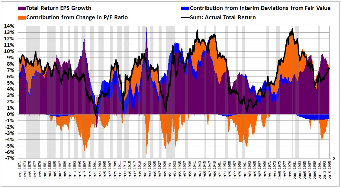
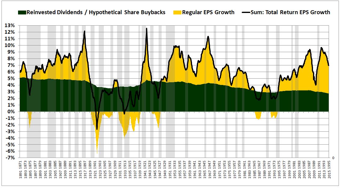
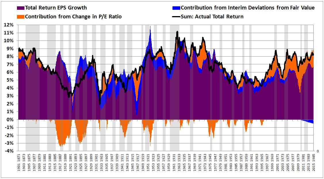
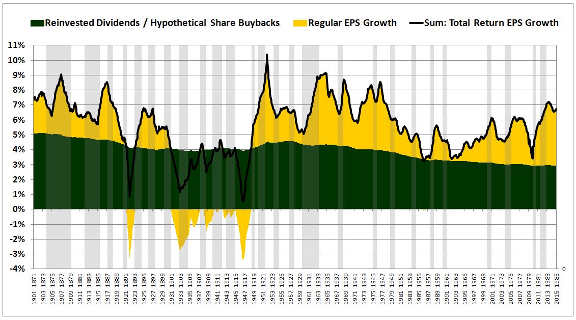
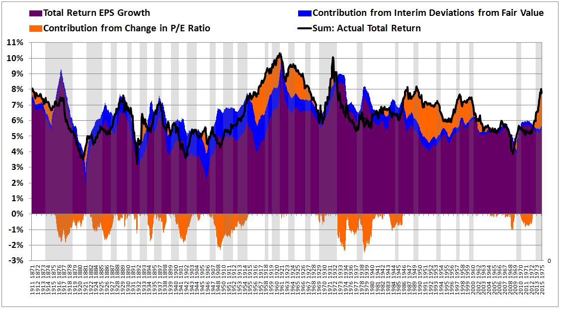
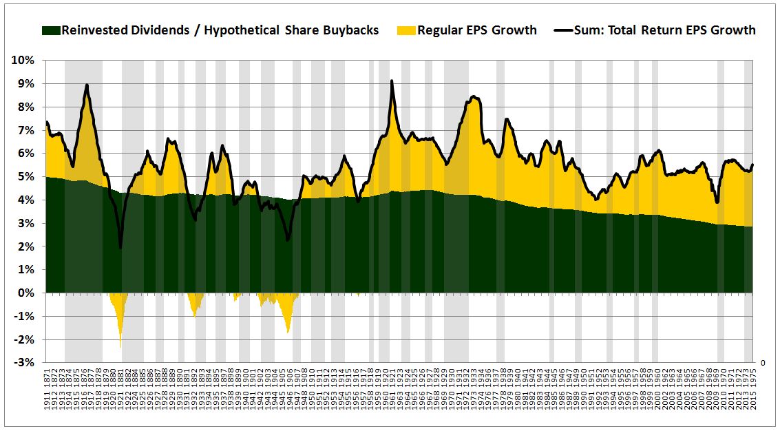
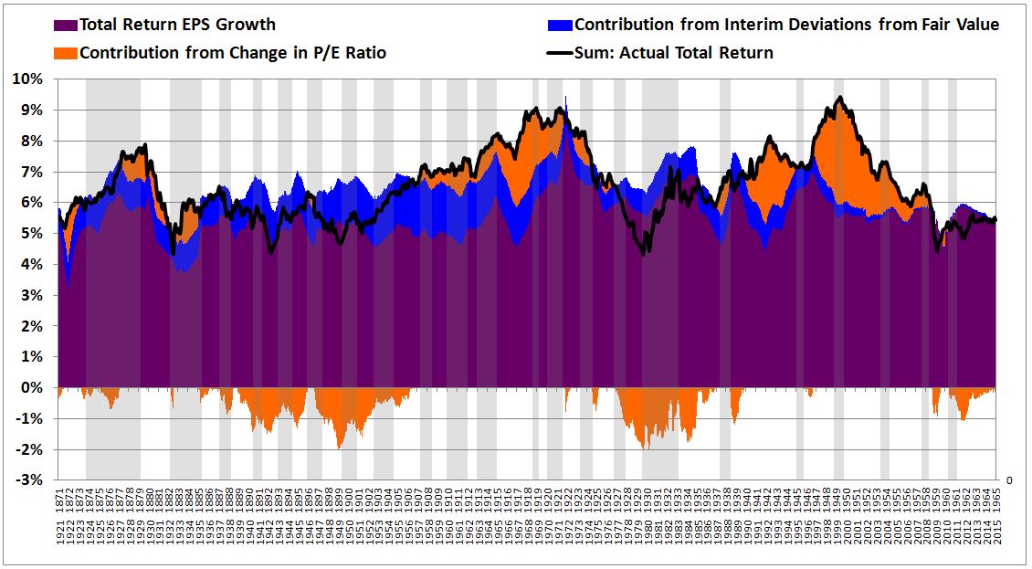
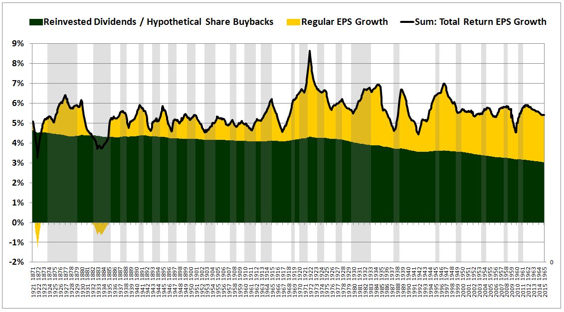
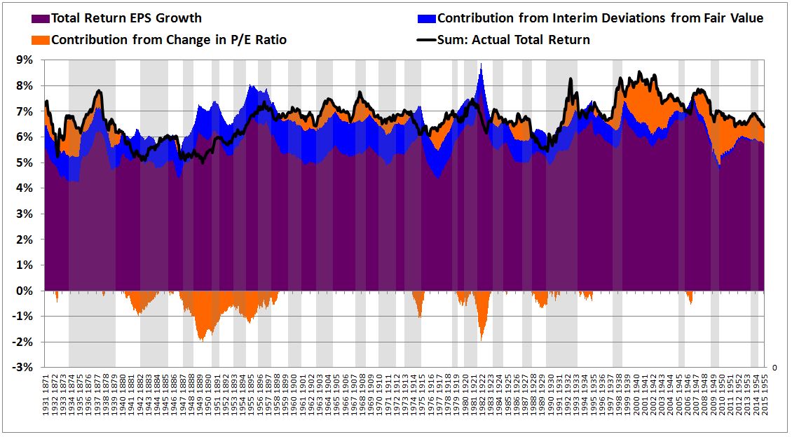
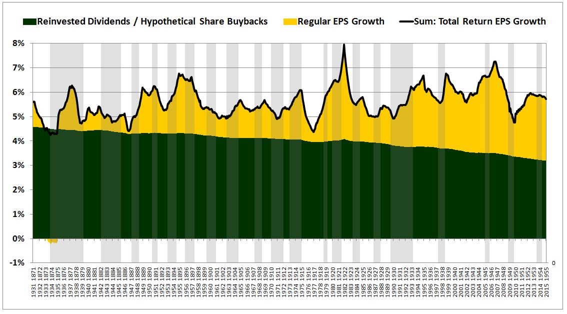
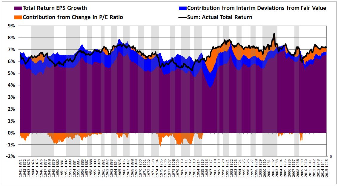
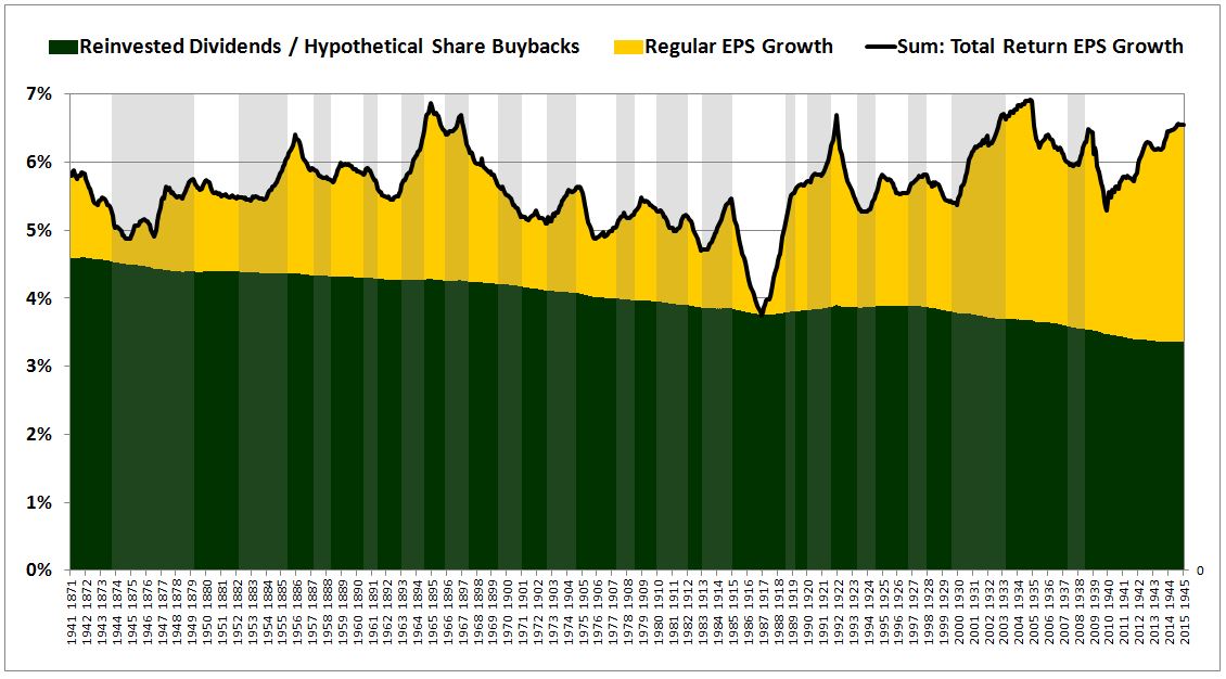
In the following charts, I’m going to decompose–i.e., separate out–the historical S&P 500 total return into three contributing components: Total Return EPS Growth (purple), Return Contribution from Change in P/E Ratio (orange), and Return Contribution from Interim Deviations from Fair Value (blue).  I’m going to further decompose Total Return EPS Growth into two components: Return from Reinvested Dividends (identical to Return from Hypothetical Share Buybacks) (green) and Regular EPS Growth (yellow). Recessionary periods for the U.S. economy will be shaded in gray.

The decompositions will be conducted on the returns at time horizons of 10, 20, 30, 40, 50, 60, and 70 years, from 1871 to 2015.  For each time horizon, there will be two separate charts (miniatures shown below), with the first chart decomposing the total return, and the second chart decomposing the Total Return EPS.  As with all numbers in this piece, the growth rates and returns are real, properly adjusted for inflation.

10 Years

A brief discussion on how to read the chart.  The x-axis has two dates.  The upper is the starting date for a period, the lower is the ending date–in this case, 10 years later.

Consider the slice of the chart that begins with 1989 and ends with 1999.  I’ve boxed it in red below:

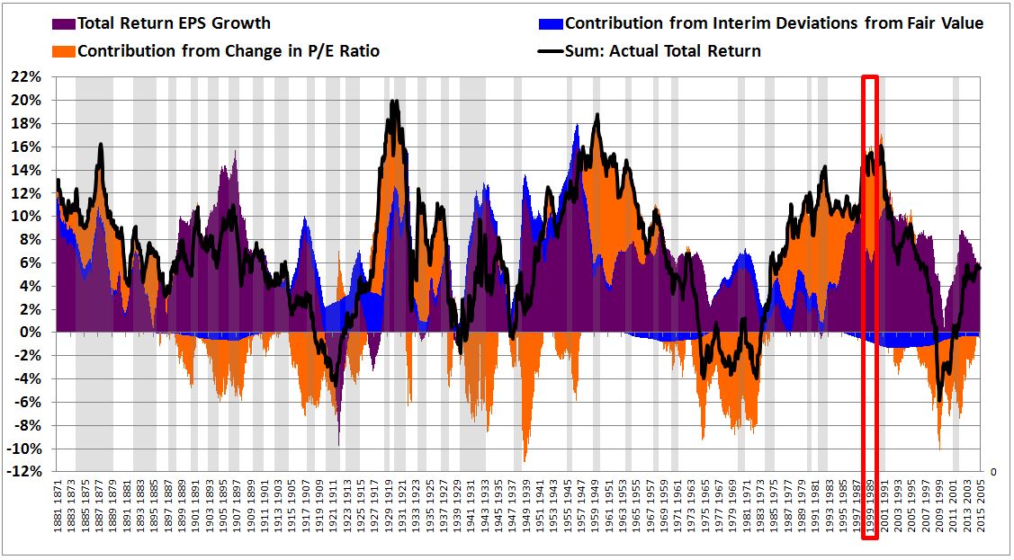
The purple, the Total Return EPS growth, was roughly on par with the historical average, around 6%. What this means is that from 1989 to 1999, the sum of the return from dividend reinvestments (or hypothetical share buybacks–same thing) at fair value and the return from regular EPS growth amounted to 6% per year.

The orange, the Contribution from the Change in P/E ratio, was enormously positive, adding more than 10% to the return.  Of course, that’s consistent with what we remember. In 1989, valuations were reasonable; in 1999, they were in a bubble.  The transition from normal valuations to bubble valuations produced phenomenal returns for shareholders. In hindsight, of course, nothing was actually “produced”–returns were simply pulled forward from the future, stolen from those that bought in at the end.

The blue, the Contribution from Interim Deviations from Fair Value, was actually negative, subtracting approximately 1% from the return.  This also checks with what we remember. From 1989 to 1999, valuations were substantially above average.  There were only a few very mild corrections that took place–certainly nothing resembling a crash.  For the most part, the market just went straight up.  The above average valuations depressed the return from reinvested dividends relative to the alternative of a market at fair value (which is what Total Return EPS is indexed to).

Notice that as we move to the right in the chart, towards starting dates in the early 1990s, the Contribution from Interim Deviations from Fair Value gets even more negative, approaching -2% per year.  To understand why, recall that the market in the late 1980s and early 1990s was actually valued fairly attractively.  When we move to the right, those years drop out, and get replaced by the acute phase of the tech bubble, when the market was radically expensive.

The thin black line is the actual total return, which almost exactly equals, within a few bps, the sum of the contributors, as it should.  Note that I’m calculating the actual total return not by summing the contributors, but by building an entirely separate total return index, using the normal methods for doing so.  The chart can therefore be taken as empirical proof that the decomposition is analytically correct–the numbers, calculated by separate methods, add up perfectly, as they should.

The chart of the decomposition of Total Return EPS, shown below, follows the same structure:

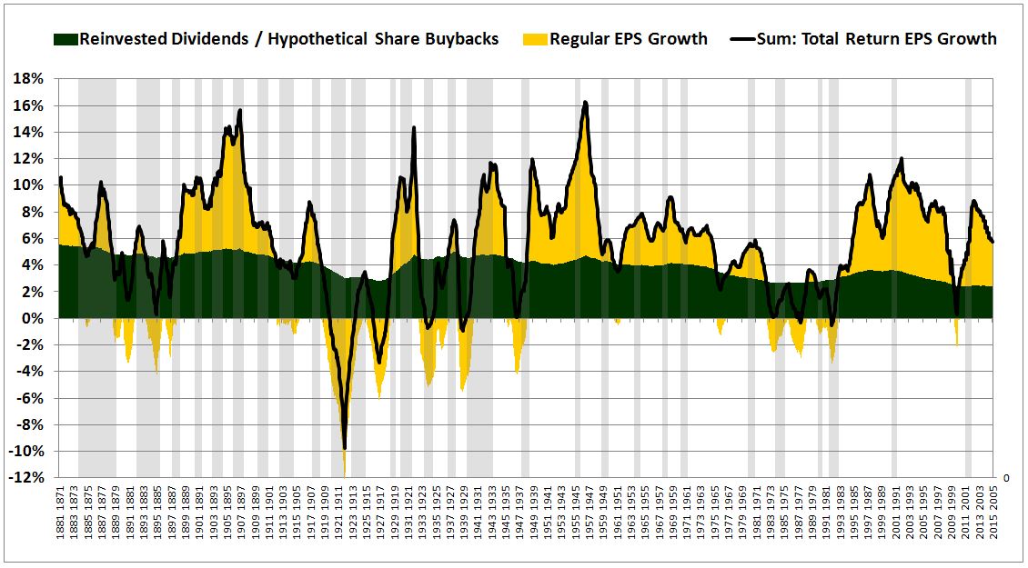
The chief thing to notice in the Total Return EPS chart is how the mix of the return has shifted from green (reinvested dividends, or alternatively, hypothetical share buybacks) to yellow (EPS growth).  This shift will become more clear and compelling as we move to longer time horizons, where the interfering cyclical noise will get smoothed out.

20 Years

30 Years

40 Years

50 Years

60 Years

70 Years

Conclusions

On longer time horizons, we see certain patterns crystallize.  The Total Return EPS, shown in purple, converges on a trend growth rate slightly below 6% annualized.  The green–the dividend (buyback) return–shrinks, while the yellow–the return from regular EPS growth–expands, keeping the sum of the two–Total Return EPS growth–on trend.

The shift from green to yellow is the shift in corporate preference visualized–away from dividends and towards growth.  When we try to conduct trend analysis on regular EPS–the yellow–we inevitably miss this shift, and therefore arrive at faulty conclusions.  What we need to analyze instead is the black line, the sum, the Total Return EPS, which has held to its trend comparatively well over the long-term.

In earlier periods of the charts, frequent market cheapness contributed meaningfully to the return.  But over time, as the market has become more efficient, less prone to violent downturns and crashes, that contribution has faded.  Notice that the blue–the contribution from interim deviations from fair value–is much thinner now than it used to be.  In charts of shorter time horizons (10 or 20 years, for example), it has even gone negative.  The shift to a negative contribution reflects the secular increase that has occurred in the market’s valuation, the valuation at which dividends are reinvested.  If, going forward, the market successfully holds steady at its currently elevated valuation, successfully avoiding the pull of downturns and crashes, then the blue will stay negative, and total returns will underperform the historical average accordingly–simply by that mechanism, never mind the others.

Investors need to understand that they can’t have it both ways: they will have to either accept historical levels of volatility, which will allow them to reinvest their dividends at cheap prices every so often (and allow their CEOs to buy back shares and acquire companies at those same prices), or they will have to accept lower than normal historical returns.  The growing corporate preference for buybacks (and acquisitions, and mergers) as a low-risk, tax-efficient alternative to risky capital expenditure will only exacerbate this impact.

At present, nearly 100% of current S&P 500 EPS is being used to fund dividends and buybacks–a trend that looks set to continue.  Going forward, interim valuations–which will influence the returns that those dividends and buybacks produce–are therefore likely to be even more impactful than they were in the past.  If valuations remain where they currently are–at levels that would qualify as historically expensive even on the uncertain assumption that profitability will remain at record highs–future returns are likely to suffer accordingly.