In prior pieces, I’ve stated that I think the S&P 500 at around 1775 can return between 5% and 6% per year over the next 10 years, a number that is significantly more attractive than the yield offered by the 10 year bond, especially after adjusting for differences in tax rates (which we have to do to be fully accurate). In what follows, I’m going to share the logic behind the estimate. I’m also going to discuss a key demographic risk to the conclusion.
Estimating Total Returns for Equities
Some analysts simplistically assume that you can accurately estimate the future total returns of equities by taking the earnings yield–the earnings divided by the price–and adding inflation. At 1775, the S&P 500 earnings yield would be around 6%. So you take 6% and add 2% for inflation to get 8% total return going forward.
But this is sloppy analysis. A stock is not a bond with a maturity. Its future returns can’t be estimated in the same way that the future returns of a 10 year bond might be estimated. In 10 years, you’re not going to get your principal back in exchange for your equities. Instead, you’re going to get back whatever price you’re able to sell your equities for, a price that the market will ultimately choose. Over the interim period, the only yield that you’re going to receive is a dividend yield. An earnings yield is not a real yield, it’s just a fictitious internal ratio. Some of it will be lost to changes in profit margins, and some of it will have to be reinvested just to keep revenues growing at the rate of inflation (and maybe even to keep revenues nominally constant).
To accurately estimate future total returns, we need to rigorously examine the individual components that drive total return. On the classic “valuation” construction, there are three components:
(1) Change in Price-Earnings (PE) Multiple
(2) Change in Earnings Per Share (EPS), consisting of:
(a) Change in Total Revenue
(b) Change in Profit Margin
(c) Change in Share Count (driven by dilution, buybacks, and acquisitions)
(3) Total Dividends Paid
If you know these three components, then you know the total return. The challenge is to estimate the path of each component over the next 10 years.
Applying the Logic Backwards to December 2003
To illustrate how an estimate of each component can yield an estimate of future total returns, let’s use the logic backwards, on the S&P 500 in December 2003. The following table shows the value each component in December 2003 and December 2013:
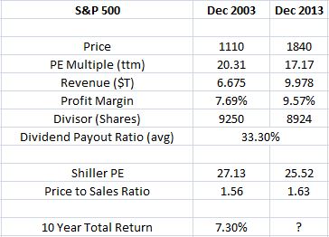
I’ve added in the Shiller PE and the Price to Sales Ratio to push back against some of the alarmist rhetoric that we’re currently hearing about “overvaluation.” The market right now is essentially at the exact same valuation that it was at in December 2003, in the early-to-middle innings of the last bull market, more than 40% below the eventual top. The 10 year total return that was earned from that point forward was a highly respectable 7.30%.
Note that we’re using the S&P 500 index divisor as an estimate of the share count. Without getting into the theoretical reasons why this is roughly accurate, and can sometimes even be conservative, suffice it to say that we can confirm the accuracy of the assumption empirically. Factset has calculated the actual change in the share count of all companies in the S&P 500 from 2004 to present. The following table shows the change alongside the change in the S&P 500 index divisor:

The two track each other relative closely, with the deviation expanding the most during the crisis period. If we assume that another 2008 crisis is not on the horizon, then the tracking error between the two should be negligible.
The strategy, then, is to take the drivers of total return (PE multiple, revenues, share count, profit margin), set them at their endpoints (2003 and 2013), and then “play” out the interim period. Each year, earnings are generated, dividends are paid and reinvested, some percentage of shares is bought back net of dilution. The revenue grows, the profit margin changes, the earnings change, the multiple changes, and so on each in an assumed linear fashion. The investor ends up with some return. The following table shows the evolution:
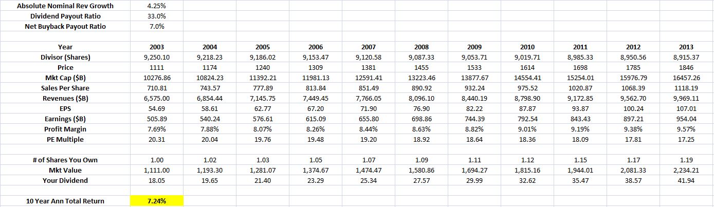
The predicted return is 7.24%, roughly equal to the actual return. Note that the numbers aren’t exact, but they shouldn’t be, as this is just an approximation.
The Change in the PE Multiple
To estimate the total return, we need to estimate the change in the PE multiple over the next 10 years. Unlike other variables that contribute to total return, the PE multiple is not set by an actual economic process. Instead, it is set by a process of portfolio allocation. The financial market presents investors with a menu of financial assets to hold–stocks, bonds, and cash. Each asset has to be held by someone. For each asset, investors push and pull on each other’s portfolios to determine who that someone will be. The PE multiple emerges as a byproduct of this process.
The question of what the PE multiple will be in 10 years is ultimately a question of how eager investors will be to own equities versus other asset classes. Trivially, the answer will depend on the sentiment towards each asset class. Sentiment is driven by a myriad of factors–the phase of the business cycle, extrapolated past experiences, expectations about interest rates, and so on.
Where in the business cycle will we be in exactly 10 years? What will the recent experiences of investors have been? Will the ride have been smooth relative to the last 10 years, or will investors have been forced to endure another ugly crash? What will expectations about the Fed’s interest rate path be? These questions are crucial to the trajectory of the PE multiple. They are very difficult to confidently answer.
Given that the current PE multiple is not particularly elevated, and that the structural forces behind low interest rates are likely to persist (as they have for the last 20 years), the best estimate for the PE multiple is probably one that doesn’t assume a large change in either direction.
At 1775, the S&P 500’s PE multiple on trailing earnings is 16.59. We’re going to assume that over the next 10 years it’s going to mean revert. But not to the average of the last 50 or 100 or 200 years, which would be an aggressive and unreasonable assumption. Rather, we’re going to assume mean reversion to the average of the last 10 years. The last 10 years excludes the overvaluation of the Tech Bubble, and includes the undervaluation of the Great Recession. It is a therefore a conservative data set to use. Conveniently, from 4Q 2003 to 4Q 2013, the geometric average PE multiple on trailing S&P operating earnings was 16.69, roughly what it is now.
The Change in the Profit Margin
To estimate what the profit margin of the S&P 500 will be in 10 years, we’re going to once again assume that mean reversion takes place. But again, we’re not going to assume mean reversion to the average of the last 50 or 100 or 200 years, which would be aggressive and unreasonable. Instead, we’re going to assume mean reversion to the average of the last 10 years.
From 4Q 2003 to 4Q 2013, the geometric average net profit margin on S&P operating earnings was 7.89%. We’re going to assume that over the next 10 years, the net profit margin will contract from its current value of 9.57% to that value, creating a meaningful drag on EPS growth.
Now, is it fair to the valuation bears to exclude all of the historical data prior to 2003 in the analysis? It doesn’t matter. The goal isn’t to be fair. The goal is to get the estimate right. People often assume that the best way to conduct a mean reversion analysis is to utilize a data set that goes as far back as you can take it. But when you take a data set back farther than its applicability warrants, you introduce data points into the analysis that are not reflective of present and likely future conditions. The polluted result ends up being less accurate, not more accurate.
The data set of the last 10 years adequately reflects how profit margins are likely to evolve in a low growth, low inflation, low interest rate, weak labor share environment–the kind of environment that has persisted in the United States for more than two decades, and that will likely continue to persist going forward. It offers a much more prudent data set for analysis than data taken from periods when the S&P 500 was dominated by “old economy” industries, when interest rates were sky high, and when labor unions ruled the day.
Crucially, our assumption represents a reasonable “middle ground” in the debate about profit margins. It acknowledges that some mean reversion will take place, but it doesn’t call for dramatic mean reversion. The level that it uses as an “average” is taken from a 10 year period that included significant economic strain.
If profit margins were “destined” to revert to 4% or 5% for the long-term, this reversion would have already happened. The economic strain of the Great Recession provided ample opportunity for it to happen. But it didn’t happen, despite continuous warnings from valuation bears that it would. This important feedback from reality needs to be respected and incorporated.
Total Revenue Growth, Share Count Change, and Dividends Paid
We need to estimate the likely growth in the total revenue (not per share) of all 500 companies in the S&P over the next 10 years. To that end, we might think that we can just use the average nGDP growth of the last 50 or 100 or 200 years, and project that average out into the future. But this approach would involve the same error that we’ve been criticizing the valuation bears for: naively assuming mean reversion to a distant past average. An indiscriminate average of the past does not necessarily represent what is likely for the future. This is especially true with respect to growth: the current potential growth rate of the U.S. economy is nowhere near the average of the last 50 or 100 or 200 years. If we project that average out in our calculation, we’re going to get an overly bullish result.
It’s important to remember that revenue growth is not free. For the corporate sector to grow at the rate of nGDP, it needs to invest in new capacity. That investment requires a diversion of cash flow that would otherwise be used to pay dividends and buy back shares. It may even require the corporate sector to conduct net share issuances. So when it comes to these variables–revenues, buybacks, dividends–we can’t just make arbitrary, independent estimates for each. We have to tie them together in the analysis. How much is the corporate sector going to devote to dividends? How much is it going to devote to share buybacks? The answer will end up being inversely proportional to the amount of revenue growth that it will be able to claim and capture.
Fortunately, there’s a simple way to conservatively and accurately estimate all three components together: revenue growth, share count change, to include the effect of dilutions, and dividends paid over the next 10 years. Just use the realized value for each variable over the last 10 years. We know that the realized values of the last 10 years are mutually achievable in practice because they actually were achieved together, despite highly unfavorable economic conditions.
The last 10 years is conservative with respect to revenue growth because it involved a deep recession and a slow recovery. It’s conservative with respect to share count change because the crisis forced large dilutions that negated most of the prior buyback gains. It’s conservative with respect to dividends because dividends were cut significantly–especially for the traditionally dividend-centric banking sector. None of these penalties needs to be incurred over the next 10 years, but to be conservative, we’ll assume they will be.
A Conservative Estimate – 5%
From 4Q 2003 to 4Q 2013, the average annual revenue growth rate for companies of the S&P 500, unadjusted for share count change, was roughly 4.25%. Note, this is nominal revenue growth, including inflation, and should not be confused with real GDP growth, which is typically much lower. The 4.25% nominal growth rate that the S&P 500 achieved over the last 10 years was significantly below the post-war average of 6% to 7%.
After adding dilution, the share count shrank by an amount that would have been equivalent to the corporate sector devoting 7% of its annual earnings to share buybacks each year. In truth, the corporate sector devoted much more to buybacks than that, but a significant portion was lost to the share dilution of the crisis, and also stock option exercise (which, unfortunately, is being unavoidably double-counted here, since it is also subtracted from operating earnings as a separate expense).
The average dividend payout ratio was around 33%. If we assume that those values hold over the next ten years, and incorporate our assumptions about the change in PE ratio (16.59 to 16.69) and the contraction in profit margins (9.57% to 7.89%), we get the following result:

The result is a 5% total return from December 2013 to December 2023. The S&P 500 starts at 1775 and ends at 2329. In absolute terms, the return is nothing to jump at, but it’s significantly better than the returns offered by cash and treasury bonds. The excess return is especially attractive when we adjust for taxes–which we have to do in order to make the analysis fully accurate. The interest payments on cash and bonds are taxed north of 40%, the capital gains and dividend payments offered by equities are taxed at 20%. At around 2.8%, the after tax yield to maturity on a 10 year treasury bond right now is around 1.7%, whereas the S&P 500 after tax total return is around 4% (assuming the highest Federal tax bracket for each).
Now, if you take the name plate yields on lower grade securities, such as junk bonds, the implied returns look higher than 5% right now–but you have to remember that we’re estimating returns across an entire credit cycle, to include a deep recession that will push default rates significantly higher. If you incorporate the impact of higher default rates, the eventual total return on junk bonds will be meaningfully less than 5%.
Importantly, our estimate is conservative. It assumes no PE multiple expansion, which could easily happen. It assumes a meaningful contraction in the profit margin, back to the levels of 2003, which doesn’t have to happen. And it uses a revenue growth rate and an assumption about dilution that was derived from a period that was sullied by a deep recession and a financial crisis, neither of which are likely to occur again in the next 10 years. Importantly, the profit margin is assumed to contract, but no additional growth is added on in exchange for that contraction, making the approach doubly conservative. Even with these penalties, the return ends up being defensible.
To give some perspective, if we added 100 bps to total annual growth, we get 6% total returns. If, in addition, we use the net buyback payout ratio of 25% that the corporate sector achieved from 2003 to 2008, before the extreme dilution of the crisis took place, we get a 7% total return. So there is plenty of upside to the 5% estimate, even on reasonable assumptions.
Now, some would point out that a 5% return over the next 10 years doesn’t mean a straight line, and that significant losses may still occur. This is true, and it’s borne out in the 2003 example. There was an attractive total return, but also a large drawdown that investors had to endure along the way.
But it’s important to remember that the point cuts both ways. Just as there may be a big drawdown over the next 10 years, there may also be a big “melt up”–a period where the market latches onto the optimism of the current growth acceleration, and rises faster than it should over the next few years, eventually overshooting its assumed final destination (S&P 500 2329 in the year 2023). It would then give back the overshoot during a subsequent contraction, resulting in a cumulative 5% total return. Given where we presently are in terms of the business cycle and monetary policy, such an outcome would seem significantly more likely right now than one where stocks spontaneously suffer a large drawdown for no reason.
The fact that long-term returns do not occur in a straight line is the very reason why, within an “acceptable” range of valuation, it’s best to focus on the business cycle, monetary policy, and price trend when investing. “Valuation” is useful more as a secondary consideration that becomes primary when it reaches clear extremes. Inside acceptable ranges, it’s not going to tell you what to do as an investor, when you need to know what to do.
Risk to the Estimate — Demographics
The estimate assumes a profit margin contraction from 9.57% to 7.89%, the average of the last 10 years. If we were to see a deeper contraction, the total return would fall significantly. For example, if the profit margin were to mean revert to the average of the last 50 years, around 5%, the total return would fall to 1%. But a profit margin contraction from 9.57% to 5% is a very aggressive assumption, discredited by the actual experience of the last 20 years. In the present low growth, low inflation, de-unionized corporate operating environment, there is no mechanism for labor to take such a sizeable share of income away from capital.
A bigger risk to the estimate, in my opinion, is demographic. Over the next 10 years, the population is set to age significantly. We don’t know how the aggregate investor preference for equities might change during that process. It’s certainly possible that the investment population, given its increasing age, could become more averse to the increased risk of equities, which would push the PE multiple down and depress the total return. For perspective, if the PE multiple were to fall to 10 over the next 10 years, from its present value of around 16, the S&P 500 total return would go from 5% to zero.
There are three reasons why I’m not especially concerned about demographic risks to the estimate. First, much of the wealth in America is concentrated in the hands of the extremely wealthy. As they grow older, the owners of that wealth are not planning to use it to fund actual retirement living expenses, but to grow it and bequeath it to heirs. Their ability and willingness to tolerate the risk of equities, in exchange for the much greater long-term return, is therefore larger than assumed. This is especially true when you consider how the money is actually managed–it’s not managed directly by the families, but by investment banks, family offices, hedge funds, and so forth.
Second, equities have earned a significant amount of goodwill among America’s older generation of wealthy individuals–the group that currently owns the majority of U.S. stocks. The buoyant equity markets of the last 30 years have been the number one causal drivers of their rising levels of wealth. That earned “goodwill” is likely to be maintained going forward, especially in an environment where the other options–cash and bonds–are offering unacceptable returns.
Third, and most importantly, as long as cash interest rates remain zero, older investors that want a return on their money will have little choice but to accept mark-to-market risk in equities. Granted, they can invest in long-term bonds, but as we saw last year, that asset class offers its own uncertainty and mark-to-market risk, particularly in environments like this one where interest rates are low and rising.
My own informal sampling of older investors suggests that they are quite comfortable owning the $JNJ’s, $PG’s, and $XOM’s of the world, names that they trust. Indeed, most of them wished they owned more, and would like to buy more if given a chance. Ironically, what they seem to be most afraid of is owning long-term bonds. They fear the effects that higher interest rates will have on their portfolios. As with all investors, their preference is going to be a function of the prevailing environment–how each asset class is performing, and how it has performed for them. As long as the economy and the business environment are healthy, and the blue chips of the S&P 500 are holding value as they pay out their dividends, there’s no reason why older investors should be expected to grow averse to them, or to prefer the zero returns of bank account cash in their place.
Now, if short-term interest rates rise in a meaningful way, and cash comes to offer an independently attractive return to older investors, the situation will obviously change. There’s no reason for older investors to accept the mark-to-market risk of equities and long-term bonds when they can earn commensurate returns in a savings account 100% free of all risk. For this reason, if the Fed were to take cash interest rates to levels that provide independently attractive returns, the market would pay a high price–not only in terms of downward pressure on valuations, but also in terms of the retarding impact on growth.
Personally, I don’t think it’s likely that we’ll see cash rates above 3% in the next 10 years, or even in our lifetimes. In the presence of elevated debt levels, aging demographics, falling population growth, rising wealth inequality, and secular stagnation, the U.S. economy simply cannot handle short-term interest rates that high. In the last expansion, it was barely able to handle rates above 4%. Almost as soon as the Fed hiked above that level, the yield curve inverted. It stayed inverted until the eventual result: a recession. The Fed understands the structural issues involved, and is going to be much more careful next time around.
To summarize, I see the demographic risk to equity valuations as hinging primarily on the short-term interest rate, the low level of which is currently pushing up the valuation of all asset classes. To be frank, I think the short-term interest rate is going to stay very low essentially forever, never again rising enough to create an independently sufficient return for investors. Seen in that light, I think the assumption that the multiple will stay around 16–when it could in fact continue to increase from here–is quite reasonable.