Free Banking on a Bitcoin Standard–The State Prepares its Death Blow

bitcoin

In a previous piece, we examined the inner workings of a gold-based fractional-reserve free banking system–the monetary system that was roughly used in the United States for much of the 19th century and before.  The system works as follows.  Customers deposit gold–which is the system’s actual money, legal tender–at private banks, and receive paper banknotes in exchange for it. Customers can redeem the banknotes for the gold at any time.

In such a system, the market eventually comes to accept the banknotes of credible banks as payment in lieu of payment in gold.  The banknotes become “good as gold”, operationally equivalent to the base money that “backs” them.

Importantly, banks take advantage of the fact that, on a net basis, very few banknotes actually get redeemed for gold.  This convenient fact allows them to issue a quantity of banknotes that exceeds the quantity of customer gold that they have on hand to meet redemptions.  They issue the excess banknotes as loans to borrowers in exchange for interest.  In this way, they expand the functional money supply, and make it possible for the economy to grow in a non-deflationary manner, despite being on a hard monetary standard.

A fractional-reserve free banking system with gold as the base represents a coveted Libertarian ideal because it requires no government involvement, other than the simple enforcement of contracts.  There are no complicated and cumbersome regulatory rules to follow, no externally-imposed reserve requirements or capital adequacy ratios, no interest rate manipulations on behalf of economic, corporate, and political interests, and so on.  All that the system contains are individuals, banks, and naturally-occurring gold (legal tender, base money), with the individuals and banks free to use fractional-reserve lending to “multiply” the gold into whatever quantity of circulating paper money they wish.  Consistent with the Libertarian ideal, if they screw up, they pay the consequences.  There is no lender of last resort to come in and clean up the mess, only private entities entering into contractual agreements with each other and doing the due diligence necessary to ensure that those agreements work out.

In the modern era, it is inconceivable that any serious legislative body would choose to put an economy on a fractional-reserve free banking system.  Such systems are highly unstable, prone to bank runs and severe liquidity crises, particularly during periods of heightened risk-aversion.  That’s precisely why central banking was invented–because free-banking doesn’t work.

However, it is conveivable that the private sector, working on its own, could one day put the economy on a fractional-reserve free banking system.  The most likely way for it to accomplish this feat would be through the use of a cryptocurrency such as Bitcoin. In what follows, I’m going to explain why fractional-reserve free Bitcoin banking is a necessary condition for Bitcoin to become a dominant form of money, and how the government will easily stop its emergence and proliferation.

Economic expansion in a capitalist system is built on the following process.  Individuals borrow money and invest it.  The borrowing for investment does three things.  First, it adds capital to the economy and increases the economy’s real output capacity.  Second, it expands the operational money supply.  Third, it creates new streams of monetary income.  The new streams of monetary income are used to consume the new streams of real output that the investment has made possible.  The spending of the new income streams by those who receive them creates income for those that made the investments.  That income is used to finance the borrowing, with some left over as profit to justify the investment.  The economy is thus able to “grow”–engage in a larger total value of final transactions at constant-prices–without needing to increase its turnover of money, because it has more money in it, money that was created through the process of borrowing and investing.  The relevant economic aggregates–real output capacity, money supply, income–all grow together, proportionately, in a balanced, virtuous cycle.

Crucially, for Bitcoin to evolve into a dominant form money, it needs to be the dominant form of money in each stage of this process.  If workers are going to get paid in Bitcoins, the investment that creates their jobs will need to be financed in Bitcoins.  If consumers are going to go shopping with Bitcoins, the associated Bitcoin revenues that their shopping creates will need to be distributed as wages and dividends in Bitcoins, or reinvested as Bitcoins.  And so on and so forth.  Trivially, we can’t just pick one part of this process and say “that’s going to be the part that uses Bitcoin.”  If Bitcoin is going to reliably displace conventional money, the whole package will need to use it.

To be clear, it’s possible that Bitcoins could become popular for use as a form of payment intermediation–in the way, that, say, a gift card is used.  You put money on a gift card, give it to someone as a gift, and they spend it.  When they spend it, the merchant that receives it converts it out of literal “plastic” form and back into money, by electronically zeroing it out and taking final claim of the money that was used to buy it.  In a similar way, even though the corporate recipients of spending have no reason to want Bitcoins–they don’t owe debts to bondholders in Bitcoins, salaries to workers in Bitcoins, dividends to shareholders in Bitcoins, or taxes to the government in Bitcoins–it is conceivable that they might still accept Bitcoins, given that there is a market to convert Bitcoins into what they do want: actual money.

But with a gift card, the intermediation is conducted for a clear reason–to eliminate the coldness and impersonality associated with giving cash as a gift, even though cash is always the most economically efficient gift to give.  With respect to Bitcoin, what would be the purpose of the intermediation?  Why, other than for techy shits and giggles (“Hey, look guys, I just bought a pizza with Bitcoins, isn’t that cool!”), or to hide illicit activity, would anyone bother to hassle with it?  Just use conventional money–in this case, dollars.  The fees associated with using dollars are imperceptible, hardly a reason to waste time with an intermediary, especially an intermediary that is extremely volatile and speculative in nature.  And it’s not even clear that those who use Bitcoin for intermediation will manage to escape fees.

When we talk about the proliferation of Bitcoin as a replacement for conventional money, we’re talking about something much bigger than a situation where certain people switch into and out of it for purchasing convenience.  In such an environment, the underlying dollars are still the ultimate monetary “end”–the cryptocurrency acts merely as a way of temporarily “packaging” that end for preferred transport.  Instead, we’re talking about a situation where the Bitcoin becomes the actual money, the medium through which incomes are earned and spent.

Fundamentally, such an outcome requires a mechanism through which Bitcoins can be borrowed.  If Bitcoins can be borrowed, then it will be possible for the virtuous process of borrowing and investing to grow the supply of Bitcoins at a pace commensurate with the demand to use them in commerce, and commensurate with the growth in the supply of everything else that grows in an expanding economy.  But if Bitcoins cannot be borrowed, then their supply will only be able to grow at the pace of computer mining output–a pace that, by design, is very slow (and that has to be slow, in order to prevent the currency from being excessively produced and depreciating in value), and that, unlike conventional money, has no logical or causal connection to the growth that occurs in any other economic aggregate.

If, as output and incomes grow, the supply of Bitcoins is unable to efficiently increase to sustain the increased volume of commerce conducted, then the exchange value of Bitcoin will always be appreciating relative to real things.  The continual appreciation will bring with it extreme bi-directional volatility as individuals come to expect continual appreciation, and attempt to speculate on it in pursuit of an investment return. Consequently, “money illusion”, the conflation of money in the mind of the user with the things that it can buy, will not be able to form.  Without “money illusion”, no one is going to be inclined to measure the commercial world in Bitcoin terms, and therefore nobody is going to be comfortable storing wealth in the currency.

Granted, individuals will be comfortable speculating in Bitcoin, trying to aggresssively grow and expand wealth by investing in it, but not storing wealth in it, which is a different activity entirely.  The result will be a volatile, stressful-to-hold instrument that functions more like an internet stock–say, $FB or $TWTR, except without the earnings prospects–than like cash in the bank or under a mattress, which is how money is supposed to behave.  Internet stocks can certainly rise on reflexive hype, but without the prospect of eventual income (something that Bitcoins don’t offer), they don’t stay risen.

Ironically, the extreme bi-directional price volatility will give Bitcoins the opposite characteristic of gift cards and other temporary stores, which is why they won’t even be survivable as forms of payment intermediation.  Who wants to buy a gift card, or receive payment with a gift card, that randomly increases or decreases in value by huge amounts every minute, every hour, every day?  Again, it’s conceivable that someone might want to purchase such a thing for shits and giggles–as a fun gamble of sorts–but not for serious commercial purposes.

It’s important to recognize that the vast majority of people that are buying Bitcoins are not doing so because Bitcoins removes hardships associated with conventional money. In everyday life, the people that are buying Bitcoins still use their dollar bills, their credit cards, their online bill pay, and everything else, with no real gripe or complaint.  The reason they are buying Bitcoins is to speculate.   They want to get in on a futuristic technology that they think has the potential to massively “disrupt” the financial world, creating wealth for those that invest ahead of the pack.  That is the only thing that’s “in” the current sky-high price–that expectation, held in the minds of a large number of people.  The current price is not evidence that Bitcoin has successfully solved any economic or financial problem that actually needs to be solved–expense, intermediation, value storage, whatever.  Conventional money is working just fine.

Now, to return to free banking, the natural way for Bitcoin to latch onto an expansionary mechanism that would allow it to become a dominant economic currency, and to thereby displace conventional money, would be if a free banking system based on Bitcoins, similar to what existed in the U.S. in the 19th century, were to evolve.  On such a model, banks would “hold” Bitcoins for their customers, and issue electronic deposits redeemable for Bitcoins in exchange.  Because depository Bitcoin inflows would roughly match or exceed depository Bitcoin outflows for the system as a whole, it would be possible for the banks to issue more Bitcoin deposits than exist in actual Bitcoins on reserve.  The excess deposits would then be available for use in lending, which would increase the operational Bitcoin supply in a way that would allow for credit transactions–the lifeblood of economic growth–to shift to Bitcoin in lieu of conventional money, and for price stability and an associated money illusion in the Bitcoin space to emerge.

On such a system, investors and entrepreneurs would be able to take out Bitcoin loans to build homes, buildings, factories, technologies, and so forth.  The workers that build those entities would receive the Bitcoins as new income, and spend them.  The new spending would produce Bitcoin revenues, which would turn into recurring Bitcoin interest payments to the Bitcoin lenders, recurring Bitcoin wages to the workers, recurring Bitcoin dividends for the investors and entrepreneurs, and so on.  At that point, Bitcoin will have “arrived.”

If people were so inclined, one can envision this setup producing a situation where conventional government currencies become obsolete–where no one wants to use them anymore, or has a need to.  If that happens, the Fed’s central planning, and the central planning of other central banks, will have been fully bypassed–defeated once and for all. Central banks will no longer be able to force bailouts, excessive inflation, negative real interest rates, financial repression, and so on down the throats of unwilling market participants.  The system will be a true Libertarian utopia, based on limited government, private enterprise, and personal responsibility.

Fortunately (in my view), and unfortunately (in the view of Bitcoin aficionados), legislators and policymakers can easily prevent this outcome from happening.  All they have to do is put in place a regulation that imposes a 100% reserve requirement on entities that “bank” in Bitcoins, i.e., that hold Bitcoins for customers.  Then, expansion of the Bitcoin supply through lending will be impossible, and the currency will forever remain a constrained, volatile, illiquid, wholely speculative venture, something inappropriate and improperly fitted for serious, non-speculative, non-shits-and-giggles, non-scandalous economic activity.  Those that are seeking to borrow and invest–to take the first steps in the virtuous process of economic and monetary growth–will have no reason to want to mess around with the cryptocurrency.

Which brings us to the “death blow.”  It appears that legislators and policymakers are already a few steps ahead.  The New York State Department of Financial Services, for example, recently issued a set of proposed virtual currency regulations.  Among them:

virtualccy


That line right there, if accepted into regulation, would be enough to conclusively destroy any hope of a Bitcoin monetary takeover.  It effectively sets a 100% reserve requirement for Bitcoin banks, making it imposible for the supply of Bitcoin to expand in the ways that would be necessary for the cryptocurrency to displace conventional money.

The significance of this vulnerability should not be understated or underestimated.  It’s very easy for the government to stop the proliferation of Bitcoin, and ultimately send the cryptocurrency to the graveyard of investment fads.  The government doesn’t have to resort to draconian, unpalatable, freedom-killing measures that would try to stop consenting adults from innocently trading Bitcoins amongst each other. All the government has to do is impose a full-reserve banking requirement on any institution that purports to engage in Bitcoin banking.  Far from wading into controversy, it can impose such a requirement under the seemingly noble and politically palatable auspice of “protecting” Bitcoin users from risky bank behavior, even though the requirement will have the intended side effect of eventually extincting the cryptocurrency, or at least of squashing its hopes for greatness.

Posted in Uncategorized | Comments Off on Free Banking on a Bitcoin Standard–The State Prepares its Death Blow

Supply and Demand: Untangling the Market’s Greatest Mystery

hwagnerOver the last ten years, the “collectibles” market has produced a fantastic return for investors.  According to the Knight Frank Luxury Investment Index, classic cars are up 550%, coins and stamps are up 350%, and fine wine and art are up 300%, with coveted items inside these spaces up by even greater amounts.

Why have collectibles performed so well, so much better than income earning assets like stocks and bonds?  Here’s a simple answer.  Over the last ten years, the supply of collectibles–especially those that are special in some way–has stayed constant.  In the same period, the demand for collectibles–driven by the quantity of idle financial superwealth available to chase after them–has exploded. When supply stays constant, and demand explodes, price goes up–sometimes, by crazy amounts.

For collectibles, “supply” is a crucial factor in determining price.  Often, the reason that a collectible becomes a collectible is that an anomaly makes it unusually rare, as was the case with the T206 Honus Wagner baseball card, shown above.  The card was designed and issued by the American Tobacco Company–one of the original 12 members of the Dow–as part of the T206 series for the 1909 season.  But Wagner refused to allow production of the card to proceed.  Some say that he refused because he was a non-smoker and did not want to participate in advertising the bad habit of smoking to children. Others say that he was simply greedy, and wanted to receive more money for the use of his image. Regardless, fewer than 200 issues of the card were manufactured, with even fewer released to the public, in comparison with hundreds of thousands of issuances of other cards in the series.  This anomaly turned an otherwise unremarkable card into a precious collectible that has continued to appreciate in value to this day.  The card most recently traded for $2,800,000, more than 100 times its price 30 years ago, even as baseball and baseball card collecting have waned in popularity.

A Similar Effect in Financial Assets?

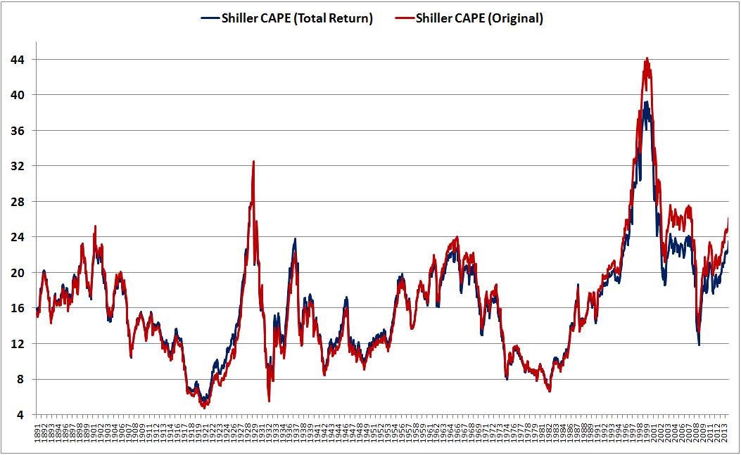
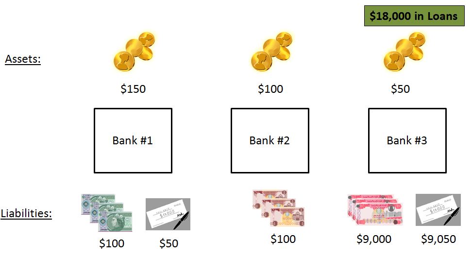
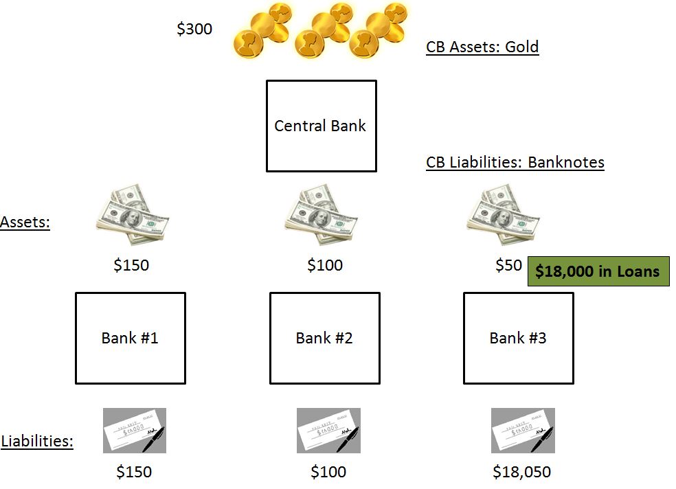
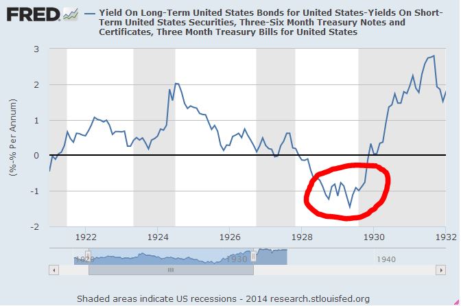
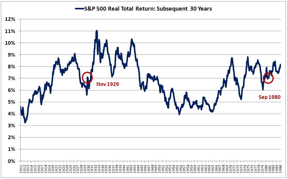
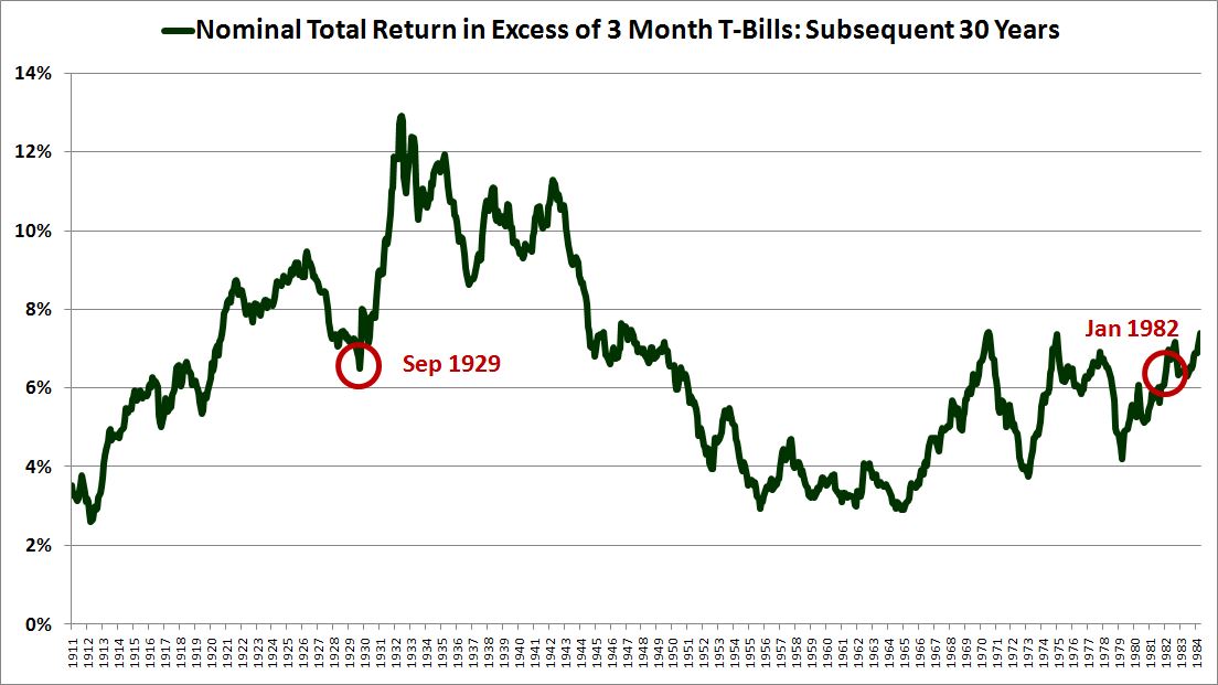
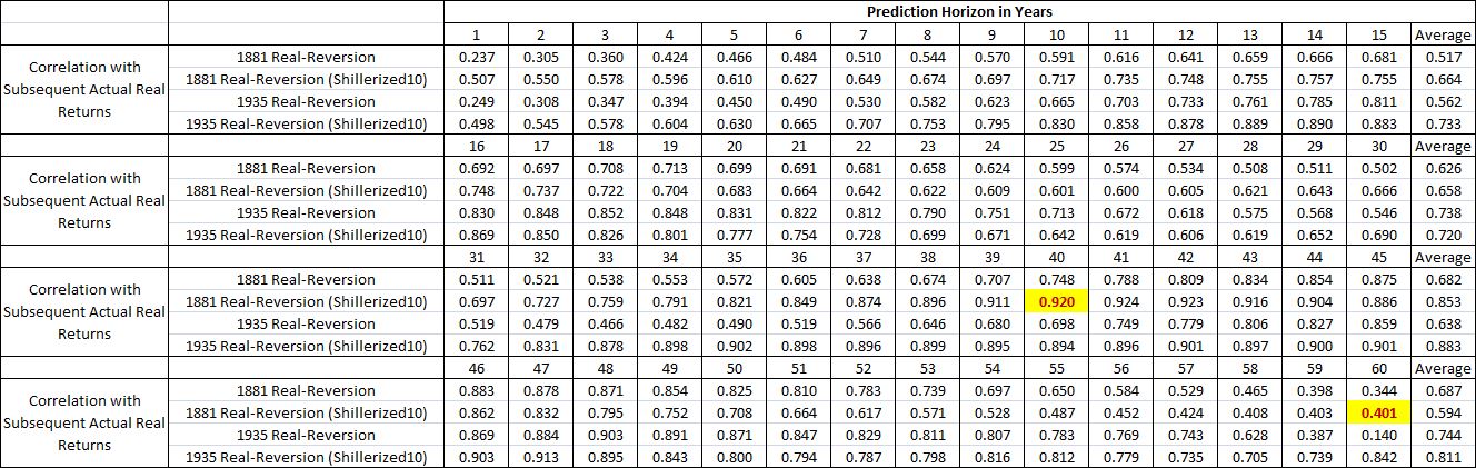
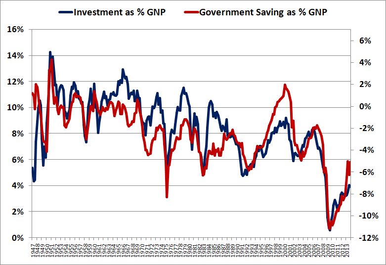
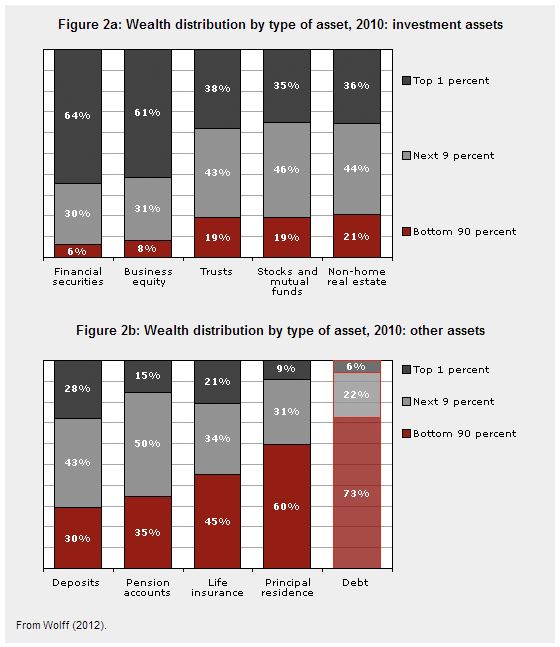
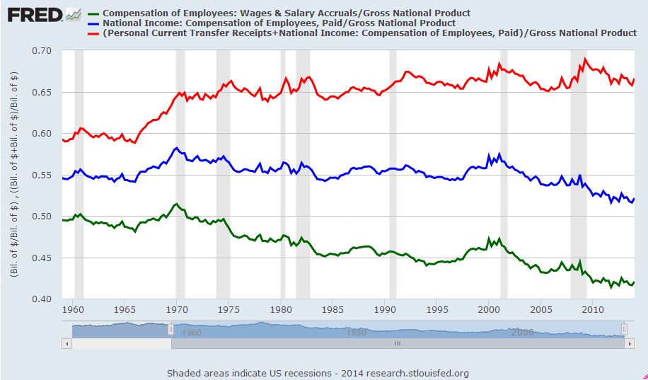
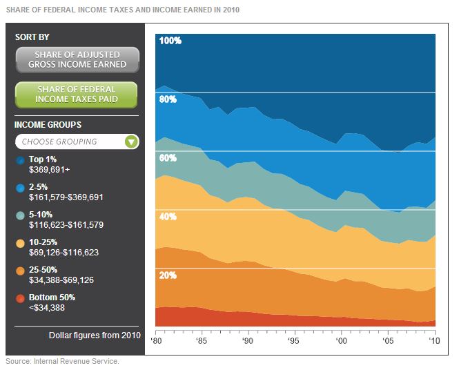
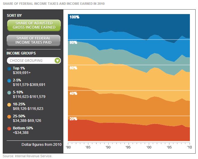
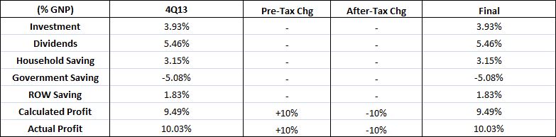
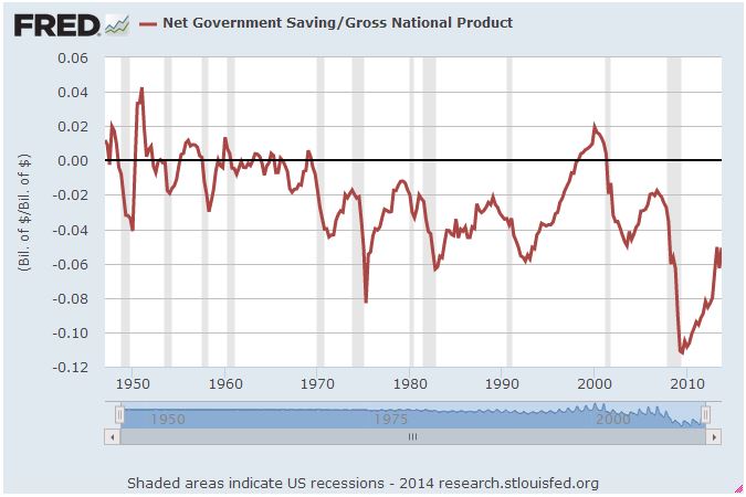
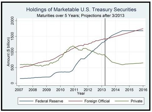
Since 2009, the Federal Reserve and foreign central banks have purchased an enormous quantity of long-term U.S. Treasury bonds.  At the same time, the quantity of idle liquidity in the financial system available to chase after these bonds has greatly increased, with central banks issuing new cash for each bond they purchase, and also offering to loan new cash to banks at near zero interest on request.  Might this fact help explain why U.S. Treasuries–and bonds in general–have become so expensive, with yields so unexplainably low relative to the strengthening U.S. growth and inflation outlook? (h/t Anti Petajisto)

tsy

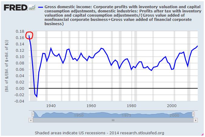
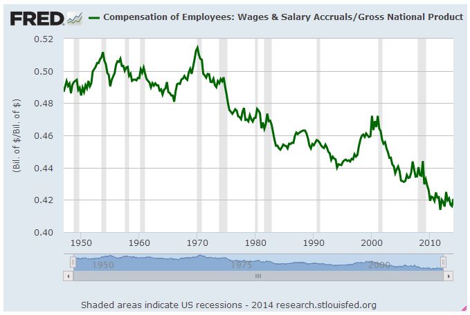
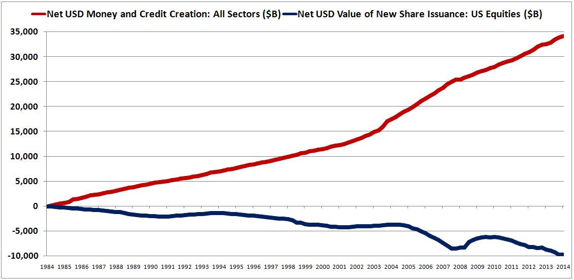
Similarly, over the last 30 years, the U.S. corporate sector has been aggressively reducing its outstanding shares, taking them off the market through buybacks and acquisitions. A continually growing supply of money and credit has thus been left to chase after a continually narrowing supply of equity.  Might this fact help explain why stocks have become so expensive relative to the past, so relentlessly inclined to grind higher, no matter the news?

mce

In this piece, I’m not going to try to answer these questions.  Rather, I’m going to present a framework for answering them.  The purpose of the framework will be to help the reader answer them, or at least think about them more clearly.

Supply and Demand: Introducing A Simple Housing Model

We often think about the pricing of financial assets in terms of theoretical constructs–“fair value”, “risk premium”, “discounted cash flow”, “net present value”, and so on.  But the actual pricing of assets in financial markets is driven by forces that are much more basic: the forces of supply and demand.  At a given market price, what amount of an asset–how many shares or units–will people try to buy? What amount of the asset–how many shares or units–will people try to sell?  If we know the answer to these questions, then we know everything there is to know about where the price is headed.

To sharpen this insight, let’s consider a simple, closed housing market consisting of some enormously large number of individuals–say, 10 billion, enough to make the market reliably liquid. Each individual in this market can either live in a home, or in an apartment.  The rules for living in homes and apartments are as follows:

(1) To live in a home, you must own it.

(2) If you own a home, you must live in it.

(3) Only one person can live in a home at a time.

(4) A person can only own one home at a time.

(5) New homes cannot be built, because there is no new land to support building.

(6) Whoever does not live in a home must live in an apartment.

(Note: We introduce these constraints into the model not because they are realistic, but because they make it easier to extend the model to financial assets, which we will do later.)

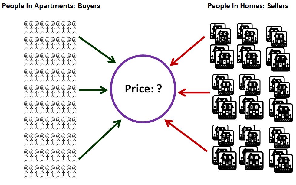
Now, let’s suppose that the homes are perfectly identical to each other in all respects. Furthermore, let’s suppose that each of the homes has already been purchased, and already has an individual living inside it. Finally, let’s suppose that there is a sufficient supply of apartment space available for the total number of people that are not in homes to live in, and that the rent is stable and cheap.  But the apartments aren’t very nice.  The homes, in contrast, are quite nice–beautiful, spacious, comfortable. Unfortunately, there are only 1 billion homes in existence, enough for 10% of the individuals in the economy to live in.  The other 9 billion individuals in the economy, 90%, will have to accept living in apartments, whether they want to or not.

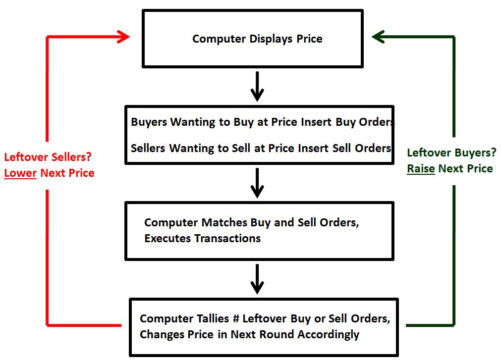
At any given moment, some number of people in homes that want to collect cash and downgrade into apartments are going to try to sell.  Conversely, some number of people in apartments that want to spend the money to upgrade are going to try to buy.  The way the market executes transactions between those that want to buy and those want to sell is as follows.  At the beginning of every second, a computer, remotely accessible to all members of the economy, displays a price.  Those that want to buy homes at the displayed price send buy orders into the computer.  Those that want to sell homes at the displayed price send sell orders into the computer.  Note that these orders is are orders to transact at the displayed price.  It’s not possible to submit orders to transact at other prices.  At the end of the second, the computer takes the buy orders and sell orders and randomly matches them together, organizing transactions between the parties.

buysellers

Now, here’s how the price changes.  If the number of buy orders submitted in a given second equals the number of sell orders, or if there are no orders, then the price that the computer will display for transaction in the next second will be the same as in the previous second.  If the number of buy orders submitted in a given second is greater than the number of sell orders, such that not all buy orders get executed, then the computer will increase the price displayed for transaction in the next second by some calculated amount, an amount that will depend on how many more buy orders there were than sell orders.  If the number of buy orders submitted in a given second is less than the number of sell orders, then the same process happens in the opposite direction.

bs

The purpose of this model is to provide a useful approximation of the price dynamics of actual markets.  The key difference between the model and a real market is that the model constrains buyers and sellers such that they can only offer to buy or sell at the displayed price, with the displayed price changing externally based on whether an excess of buyers or sellers emerges.  The reason we insert this constraint is to make the market’s path to equilibrium easy to conceptually follow–the path to equilibrium proceeds in a step by step manner, with the market trying out each price, and moving higher or lower based on which flow is greater at that price: buying flow or selling flow.  But the constraint doesn’t change the eventual outcome.  The price dynamics and the final equilibrium price end up being similar to what they would be in a real market where investors can accelerate the market’s path to equilibrium by freely shifting bids and asks.

Unpacking the Model: The Price Equation

The question we want to ask is, at what price–or general price range–will our housing market eventually settle at?  And if prices are never going to settle in a range, if they are going to continually change by significant, unpredictable amounts, what factors will set the direction and magnitude of the specific changes?

To answer this question, we begin by observing that the displayed price will change until a condition emerges in which the average number of buy orders inserted per unit time at the displayed price equals–or roughly equals–the average number of sell orders inserted per unit time at the displayed price.  Can you see why?  By the rules of the computer, if they are not equal, the price will change, with the magnitude of the change determine by the degree of unequalness.  So,

(1) Buy_Orders(Price) = Sell_Orders(Price)

“Price” is in parentheses here to indicate that the average number of buy orders that arrive in the market per unit time and the average number of sell orders that arrive in the market per unit time are functions of the price.  When the price changes, the average number of buy orders and sell orders changes, reflecting the fact that buyers and sellers are sensitive to the price they pay.  They care about it–a lot.

Now, we can separate Buy_Orders(Price), the average number of buy orders that occurs at a given price in a given period of time, into a supply term and a probability term.

Let Supply_Buyers be the supply term.  This term represents the number of potential buyers, which equals the number of individuals living in apartments–per our assumptions, 9 billion.

Let Probability_Buy(Price) be the probability term.  This term represents the average probability or likelihood that a generic potential buyer–any unspecified individual living in an apartment–will submit a buy order into the market in a given unit of time at the given price.

Combining the supply and probability terms, we get,

(2) Buy_Orders(Price) = Supply_Buyers * Probability_Buy(Price)

What (2) is saying is that the average number of buy orders that occurs per unit time at a given price equals the supply of potential buyers times the probability that a generic potential buyer will submit a buy order per unit time, given the price.  Makes sense?

Now, we can separate Sell_Orders(Price) in the same way, into a supply term and a probability term.  Let Supply_Homes be the supply term–per our assumptions, 1 billion.  Let Probability_Sell(Price) be the probability term, with both terms defined analogously to the above.  Combining the supply and probability terms, we get,

(3) Sell_Orders(Price) = Supply_Homes * Probability_Sell(Price)

(3) is saying the same thing as (2), except for sellers rather than buyers.  Combining (1), (2), and (3), we get a simple and elegant equation for price:

(4) Supply_Buyers * Probability_Buy(Price) = Supply_Sellers * Probability_Sell(Price)

The left side of the equation is the flow of attempted buying.  The right side of the equation is the flow of attempted selling.  The price that brings the two sides of the equation into balance is the equilibrium price, the price that the market will continually move towards. The market may not hit the price exactly, or be able to remain perfectly stable on it, but if the buyers are appropriately price sensitive, it will get very close, hovering and oscillating in a tight range.

The Buy-Sell Probability Function

Now, we know how many potential buyers–how many apartment dwellers–the market has: 9 billion.  We also know how many potential sellers–how many homes and homeowners–the market has: 1 billion.  9 billion is nine times 1 billion.  It would seem, then, that the market will face a permanent imbalance–too many buyers, too few sellers. But we’ve forgotten about the price.  As the price of a home rises, the portion of the 9 billion potential buyers that will be willing to pay to switch to a home will fall.  These individuals do not have infinite pocket books, nor do they have infinite supplies of credit from which to borrow.  Importantly, paying a high price for a home means that they will have to cut back on other expenditures–the degree to which they will have to cut back will rise as the price rises, making them less likely to want to buy at higher prices.

Similarly, as the price rises, the portion of the 1 billion homeowners that will be eager to sell and downsize into apartments will rise.  In selling their homes, they will be able to use the money to purchase other wanted things–the higher the price at which they sell, the more they will be able to purchase.

This dynamic is what the buy-sell probability functions, Probability_Buy(Price) and Probability_Sell(Price), are trying to model.  Crucially, they change with the price, increasing or decreasing to reflect the increasingly or decreasingly attractive proposition that buying and selling becomes as the price changes.  By changing with price, the terms make it possible for the two sides of the equation, the flow of attempted buying and selling, to come into balance.

Now, what do these functions look like, mathematically?  The answer will depend on a myriad of factors, to include the lifestyle preferences, financial circumstances, learned norms, past experiences, and behavioral propensities of the buyers and sellers.  There is some price range in which they will consider buying a home to be worthwhile and economically justifiable–this range will depend not only on their lifestyle preferences and financial circumstances, but also, crucially, on (1) the prices they are anchored to, i.e., that they are used to seeing, i.e., that they’ve been trained to think of as normal, reasonable, versus unfair or abusive, and (2) on what their prevailing levels of confidence, courage, risk appetite, impulsiveness, and so on happen to be.  Buying a home is a big deal.

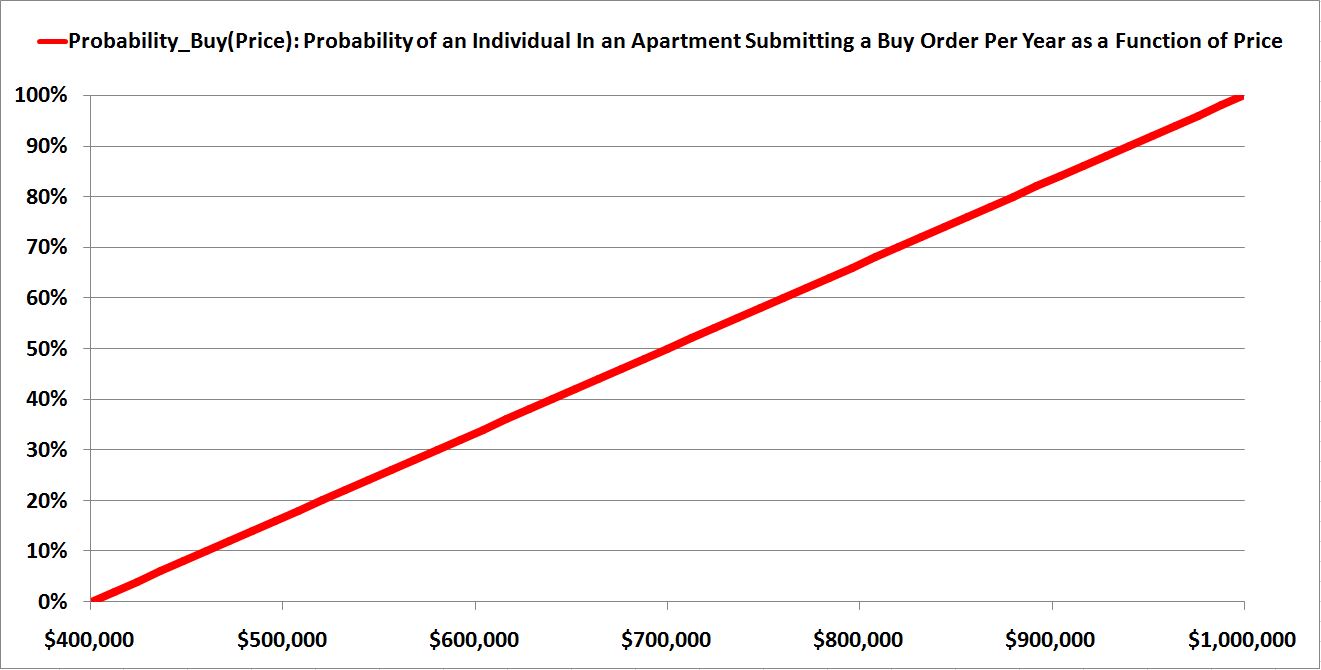
For buyers, let’s suppose that this price range begins at $0 and ends at $500,000.  At $0, the average probability that a generic potential buyer–any individual living in an apartment–will submit a buy order in a given one year time frame is 100%, meaning that every individual in an apartment will submit one buy order, on average, per year, if that price is being offered (to change the number from per year to per second, just divide by the number of seconds in a year).  As the price rises from $0 to $500,000, the average probability falls to 0%, meaning that no one in the population will submit a buy order at $500,000, ever.

In “y = mx + b” form, we have,

(5) Probability_Buy(Price) = 100% – Price * (100%/$500,000)

The function is graphed below in green:

buyfunct

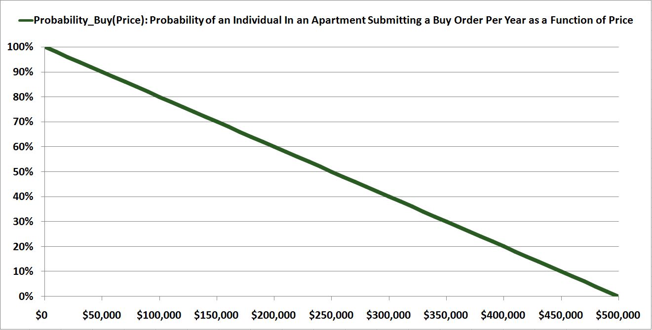
Notice that the function is negatively-sloping.  It moves downward from left to right.

For sellers, let’s suppose that the price range begins at $1,000,000 and ends at $400,000. At $1,000,000, the average probability that a generic potential seller–any individual living in a home–will submit a sell order in a given one year time frame is 100%.  As the price falls to $400,000, the average probability falls to 0%.

In “y = mx + b” form,

(6) Probability_Sell(Price) = Price * (100%/$600,000) – 66.6667%

The function is shown below in red:

psell

Notice that the function is positively-sloping.  It moves upward from left to right.

Knowing these buy-sell probability functions, and knowing the number of individuals in apartments and the number of individuals in homes (the supplies that the probabilities will be acting on, 9 billion and 1 billion, respectively), we can plug equation (5) and equation (6) into equation (4) to calculate the equilibrium price.  In this case, the price calculates out to roughly $491,525 for a home.  The average probability of buying per individual per unit time will be low enough, and the average probability of selling per individual per unit time high enough, to render the average flow of attempted buying equal to the average flow of attempted selling, as required, even as the supply of potential buyers remains 9 times the supply of potential sellers.

Notably, the turnover, the volume of buying and selling, is going to be very low, because the buy-sell probability functions overlap at very low probabilities.  The buyers and the sellers are having to be stretched right up to the edge of their price limits in order to transact, with the buyers having to pay what they consider to be a very high price to transact, and the sellers having to accept what they consider to be a very low price to transact.

Now, keeping these buy-sell functions the same, let’s massively shrink the supply of potential buyers, to see what happens to the equilibrium price.  Suppose that instead of having 9 billion individuals in the economy living in apartments, suppose that we only have 1 million individuals living in apartments–1 million potential buyers of homes, none of whom are willing to pay more than $500,000.  As before, we’ll assume that there are 1 billion homes that can potentially be sold. What will happen to the price?  The answer: it will fall from roughly $491,525 to roughly $400,119.

Notice that the price won’t fall by very much–it will fall by only roughly $90,000–even though we’re dramatically shrinking the supply of potential buyers, by a factor of 9,000. The reason that the price isn’t going to fall by very much is that the sellers are sticky–they don’t budge.  Per their buy-sell probability functions, they simply aren’t willing to sell properties at prices below $400,000, and so if there aren’t very many people to bid at prices above $400,000, because the supply of buyers has been dramatically shrunk, then the volume will simply fall off.  In the former case, with the supply of potential buyers at 9 billion, 155 million homes get sold, on average, in a one year period.  In the latter case, with the supply of potential buyers at only 1 million, 200,000 homes get sold, on average, in a one year period.

Behavioral Factors: Anchoring and Disposition Effect

Recall that for buyers, the buy-sell probability function slopes negatively–i.e., falls downward–with price.  For sellers, the function slopes positively–i.e., rises upward–with price.  The reason the function slopes negatively for buyers is that price is a cost, a sacrifice, to them.  The lower or higher the price, the higher or lower that cost, that sacrifice.  Additionally, there is a limit to the cost the buyer can pay–he only has so much money, so much access to credit. The reason the function slopes positively for sellers is that price is a benefit, a gain, to them.  The lower or higher the price, the lower or higher that benefit, that gain.  Additionally, there is a limit to the price that the seller can accept without pain, particularly if he has debts to pay against the assets that he is trying to sell.

In addition to these fundamental considerations, there are also behavioral forces that make the functions negatively-sloping and positively-sloping for buyers and sellers respectively.  Of these forces, the two most important are anchoring and disposition effect.

Over time, buyers and sellers become anchored to the price ranges that they are used to seeing.  As the price move out of these ranges, they become more averse, more likely to interpret the price as an unusually good deal that should be immediately taken advantage of or as an unfair rip-off that should be refused and avoided.

Anchoring is often seen as something bad, a “mental error” of sorts, but it is actually a crucially important feature of human psychology.  Without it, price stability in markets would be virtually impossible.  Imagine if every individual entering a market had to use “theory” to determine what an “appropriate” price for a good or service was.  Every individual would then end up with a totally different conception of “appropriateness”, a conception that would shift wildly with each new tenuous calculation.  Prices would end up all over the place.  Worse yet, individuals would not be able to quickly and efficiently transact.  Enormous time resources would have to be spent in each individual transaction, enough time to do all the necessary calculations.  This time would be spent for nothing, completely wasted, as the calculation results would not be stable or repeatable.  From an evolutionary perspective, the organism would be placed at a significant disadvantage.

In practice, individuals need a quick, efficient, consistent heuristic to determine what is an “appropriate” price and what is not.  Anchoring provides that heuristic.  Individuals naturally consider the price ranges that they are accustomed to seeing and transacting at as “appropriate,” and they instinctively measure attractiveness and unattractiveness against those ranges.  When prices depart from the ranges, they feel the change and alter their behaviors accordingly–either to exploit bargains or to avoid rip-offs.

Disposition effect is also important to price stability.  Individuals tend to resist selling for prices that are less than the prices for which they bought, and tend to be averse to paying higher prices than the prices could have paid in the recent past.  This tendency causes price to be sticky, discinlined to move away from where they have been, as we should want them to be if we want markets to hold together, and not become chaotic.

Housing markets represent an instance where these two phenomena–anchoring and disposition effect–are particularly powerful, especially for sellers.  The phenomena is part of what makes housing such a stable asset class relative to other asset classes.

homeprices

Homeowners absolutely do not like to sell their homes for prices that are lower than the prices that they paid, or that are lower than the prices that they are accustomed to thinking their homes are worth.  If a situation emerges in which buyers are unwilling to buy at the prices that homeowners paid, or the prices that homeowners are anchored to, the homeowners will try to find a way to avoid selling.  They will choose to stay in the home, even if they would prefer to move elsewhere.  If they need to move–for example, to take a new job–they will simply rent the home out; anything to avoid selling the home, taking a loss, and giving an unfair bargain to someone else.  Consequently, market conditions in which housing supply greatly exceeds housing demand tend to clear not through a fall in price, but through a drying up of volume, as we saw in the example above.

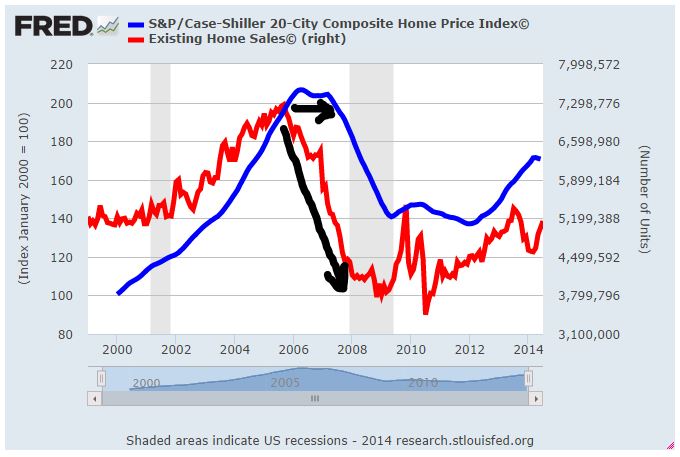
This effect was on fully display in the last recession.  Existing home sales topped out in 2005, but prices didn’t actually start falling in earnest until the recession hit in late 2007 and early 2008.  Prior to the recession, the homes were held tightly in the hands of homeowners.  As long as they could afford to stay in their homes, they weren’t going to sell at a loss.  But when the recession hit, they started losing their jobs, and therefore their ability to make their mortgage payments.  The result was a spike in foreclosures that put the homes into the hands of banks, mechanistic sellers that were not anchored to a price range and that were not averse to selling at prices that would have represented losses for the prior owners.  The homes were thus dumped onto the market at bargain values to whoever was willing to buy them.

homesales

When Is Supply Important to Price? 

Returning to the previous example, what would be the market outcome if buyers and sellers were completely insensitive to price, such that their buy-sell probability functions did not slope with price?  Put differently, what would be the market outcome if the average probability that a potential buyer or seller would buy or sell in a given unit of time–a given year–stayed constant under all scenarios–always equal to, say, 10%, regardless of the price?

The answer is that supply imbalances would cause enormous fluctuations in price.  Theoretically, any excess in the number of potential buyers over the number of potential sellers would permanently push the price upward, all the way to infinity, and any excess in the number of potential sellers relative to the number of potential buyers would permanently pull the price downward, all the way to zero.

In concrete terms, if there are 1,001 eager buyers that submit buy orders per unit time, and 1,000 eager sellers that submit sell orders, and if the buyers are completely indifferent to price, then there will always be one buyer left out of the mix.  Because that buyer is indifferent to price, he will not hesitate to raise his bid, so as to ensure that he isn’t left out of a transaction.  But whoever he displaces in the bidding will also be indifferent to price, and therefore will not hesitate to do the same, raise the bid again–and so on.  Participants will continue to raise their bids ad infinitum, continually fighting to avoid being the unlucky person that gets left out.

The only way for the process to end is for 1 of the buyers in the group to conclude, “OK, enough, the price is just too high, I’m not interested.”  That is price sensitivity.  Without it, a stable equilibrium amid a disparate supply of potential buyers and sellers cannot be achieved.

We now have the ability to answer an important question at the heart of this piece: when is “supply” most important to price, most impactful?  The answer is, when price sensitivity is low.  If the probability of buying doesn’t fall quickly in response to an increase in price, and if the probability of selling doesn’t fall quickly in response to a decrease in price, then even a small change in the supply of potential buyers or sellers will be able to create a large change in the price outcome.  In contrast, if the price sensitivity is high, if the probability of buying falls quickly in response to price increases, and the probability of selling falls quickly in response to price reductions, then the price will be able to remain steady, even in the presence of large supply excursions.  Intuitively, the reason the price will be able to remain steady is that the potential buyers and sellers will be holding their grounds–they won’t be budging off of their desired price ranges simply to make transactions happen.

Low price sensitivity is part of the reason why small speculative stocks with ambiguous but potentially exciting futures–low-float stocks with large potentials that are difficult to confidently value and that exhibit significant price reflexivity–tend to be highly volatile.  If there is a net excess or shortage of eager buyers in these stocks relative to eager sellers, the price will end up changing.  But the change will not correct the excess or shortage. Therefore the change will not stop.  It will keep going, and going, and going, and going.

To use a relevant recent example, if there is a shortage in the supply of $LOCO shares being offered in an IPO relative to the amount of $LOCO that investors want to allocate into, then the price is going to increase.  For the market in $LOCO to remain stable, this price increase will need to depress the demand, reduce the amount of $LOCO that investors want to allocate into.  If the price increase fails to depress the demand, or worse, if it does the opposite, if it increasess the demand–for example, by drawing additional attention to the name and increasing investor optimism about the company, given the rising price–then the price is going to get pushed higher and higher and higher.

At some point, something will have to reverse the process, as the price can’t go to infinity. In the case of $LOCO, more and more people might start to ask themselves, have things gone to far?  Is this stock a bubble that is about to burst?  An excess of sellers over buyers will then emerge, and the same process will unfold in the other direction.  When the price falls, the fall will not sufficiently clear the excess demand to sell, and may even increase it, by fueling anxiety, skepticism and fear on the part of the remaining holders.  And so the price will keep falling, and falling, and falling.

Now, if we shift from $LOCO IPO to a market where price sensitivity is strong, this dynamic doesn’t take hold.  To illustrate, suppose that the treasury were to issue a massive, gargantuan quantity of three month t-bills.  The same instability would not emerge.  The reason is that there is a strong inverse relationship between the price of three month t-bills and the demand to own them, a relationship held in place by the possibility of direct arbitrage in the banking system.  Recall that a three month t-bill offers a return that is fully-determined and free of credit risk.  It also carries no interest rate risk beyond a period of three months (the money will have been returned by then).  Thus, as long as the Fed holds overnight interest rates steady over the next three months, as the current Fed has effectively promised to do, banks will be able to borrow funds and purchase three month t-bills, capturing any excess return above the overnight rate that the bills happens to be offering, without taking on any risk.  And so any fall in the price of a three month treasury bill, and any rise in the yield, will represent free money to banks.  That free money will attract massive buying interest, more than enough to quench whatever increased selling flow might arise out of a large increase in the outstanding supply. Ultimately, when it comes to short-term treasuries, supply doesn’t matter much to price.

Extending the Model to Financial Assets: Equity and Credit

To extend the housing model to financial assets, we begin by noting that units of financial “wealth”–that is, units of the market value of portfolios, in this case measured in dollars–are analogous to “individuals” in the housing model.  Just as individuals could either live in homes or apartments–and had to choose one or the other–units of financial “wealth” can either be held in the form of equity (stocks), credit (bonds), or money (cash).  Just as every home had to have an owner and every apartment a tenant living inside it, every outstanding unit of equity, credit, and money in existence has to have a holder, has to be a part of someone’s portfolio, with a portion of the wealth contained in that portfolio stored inside it.

Now, to make the model fully analogous, we need to reduce the degrees of freedom from three (stocks, bonds, cash) to two (stocks, cash). So we’re going to treat bonds and cash as the same thing, referring to both simply as “cash.”  Then, investors will have to choose to hold financial “wealth” either in the form of “stocks”, or in the form of “cash”, just as “individuals” had to choose to live either in “homes”, or in “apartments.”

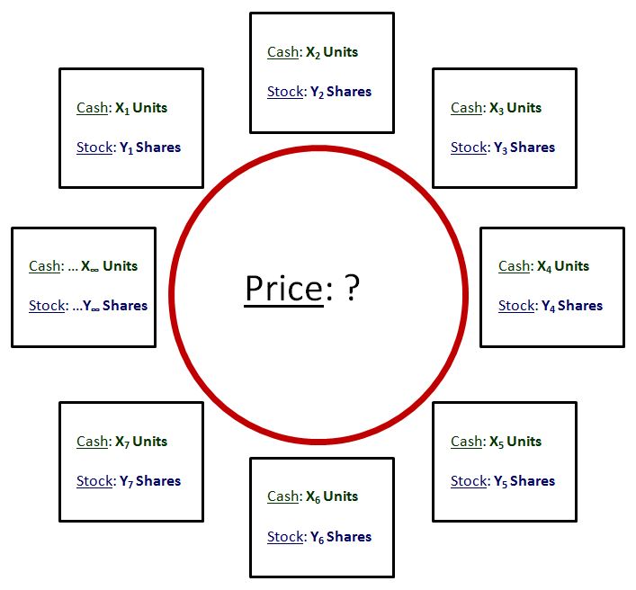
Let’s assume, then, that our stock market consists of some amount of cash–some number of individual dollars–and some amount of stock, some number of shares with a total dollar value determined by the price.  Let’s also assume that the same computer is there to take buy and sell orders–orders to exchange cash for stock or stock for cash respectively. The computer processes orders and moves the price towards equilibrium in the same way as before, by displaying a price–an exchange rate between stock and cash–then taking orders, then raising or lowering the price in the next moment based on where the excess lies.

The derivation of the price equation ends up being the same as in the housing model, and gives the following result.

(7) Supply_Cash * Probability_Buy(Price) = Supply_Stock(Price) * Probability_Sell(Price)

Here, Supply_Cash is the total dollar amount of cash in the system. Probability_Buy(Price) is the average probability, per dollar unit of cash in the system, per unit of time, that the unit of cash will be sent into the market to be exchanged for stock at the given price.  Supply_Stock is the the total market value of stock in existence. Probability_Sell(Price) is the average probability, per dollar unit of value of stock in the system, that the unit will be sent into the market to be exchanged for cash at the given price.

Now, where this model differs from the previous model is that Supply_Stock, the total market value of stock in existence, which is the total amount of stock available for investors to allocate their wealth into, is a function of Price.  It equals the number of number of shares times the price per share.

(8) Supply_Stock(Price) = Number_Shares * Price

Unlike in the housing model, the supply of stock in the stock market expands or contracts as the price rises and falls.  This ability to expand and contract helps to quell excesses that emerge in the amount of buying and selling that is attempted.  If investors, in aggregate, want to allocate a larger portion of their wealth into stocks than is available in the current supply, the price of stocks will obviously rise.  But the rising price will cause the supply of stocks–the shares times the price–to also rise, helping, at least in a small way, to relieve the pressure.  The same is true in the other direction.

Combing (7) and (8), we end up with a final form for the equation,

(9) Supply_Cash * Probability_Buy(Price) = Number_Shares * Price * Probability_Sell(Price)

Note that we’re using this equation to model stock prices, but we could just as easily use the equation to model the price of any asset, provided that simplifying assumptions are made.

A more accurate form of the equation would include a set of terms to model the possibility of margin buying and short selling.  These terms are shown in green,

(10) Supply_Cash * Probability_Buy(Price) + Supply_Borrowable_Cash * Probability_Borrow_To_Buy(Price)Number_Shares * Price * Probability_Sell(Price) + Number_Borrowable_Shares * Price * Probability_Borrow_To_Sell(Price)

But the introduction of these terms makes the equation unnecessarily complicated.  The extra terms are not needed to illustrate the underlying concepts, which is all that we’re trying to do.

A Growing Cash Supply Chases A Narrowing Stock Supply: What Happens?

It is commonly believed that the stock market–the aggregate universe of common stocks–rises over time because earnings rise over time.  Investors are sensitive to value. They estimate the future earnings of stocks, and decide on a fair multiple to pay for those earnings. When the stock market is priced below that multiple, they buy.  When the stock market is priced above that multiple, they sell.  In this way, they keep the price of the stock market in a range–a range that rises with earnings over time.

In a set of pieces from last year (#1, #2), I proposed a competing explanation.  On this explanation, the stock market rises over time because we operate in an inflationary financial system, a system in which the quantity of money and credit are always growing. Given its aversion to dilution, the corporate sector does not issue enough new shares to keep up with this growth.  Consequently, a rising quantity of money and credit is left to chase after a limited quantity of shares, pushing the prices of shares up through a supply effect.  Conveniently, as prices rise, the supply of stock rises, bringing the supply back into par with the supply of money and credit.

The truth, of course, is that both of these factors play a role in driving the stock market higher.  Which factor dominates depends on the degree of price sensitivity–or, in this case, the degree of value sensitivity–of the buyers and sellers.  In a world where buyers and sellers are highly sensitive to the price-earnings ratio, the supply effect will not exert a signficant effect on prices. Prices will track with earnings and earnings alone.  In a world where buyers and sellers are not highly sensitive to the price-earnings ratio, or to other price-based measurements of value, the supply effect will become more significant and more powerful.

We can illustrate this phenomenon by running the model computationally, with random offsets and deviations inserted to help simulate what happens in a real market.  Assume, that there are 1,000,000 shares of stock in the market, and $2B dollars of cash.  Assume, further, that each share of stock earns $100 per year in profit.  Finally, assume that the buy-sell probability functions for buyers and sellers are symmetric cumulative distribution functions (CDF) of Gaussian distributions with very small standard deviations.  These functions take not only price as input, but also earnings.  They compute the PE ratio at a given price and output a probability of buying or selling based on it.

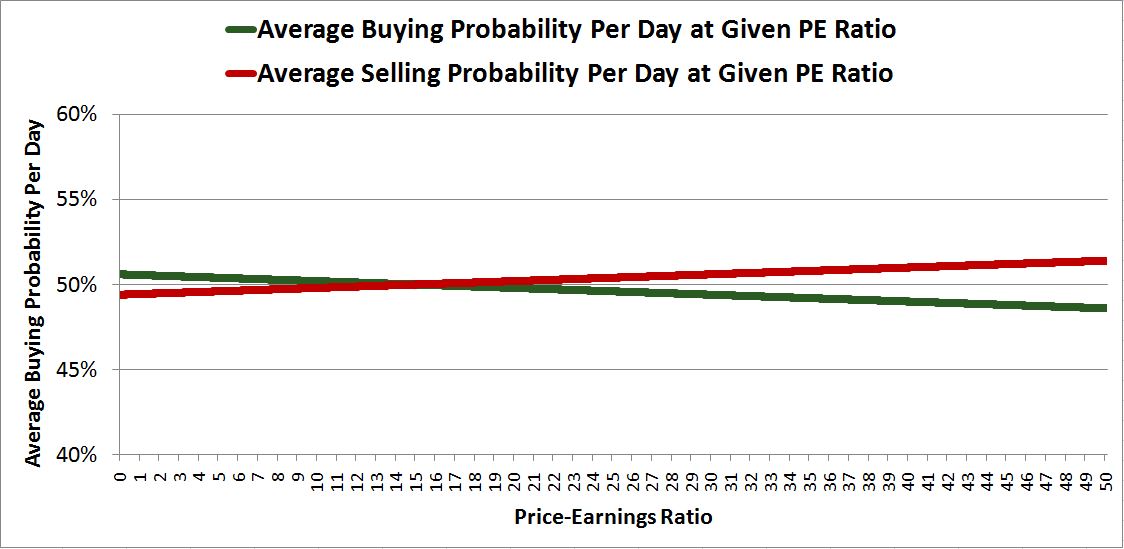
The functions look like this:

avgprob

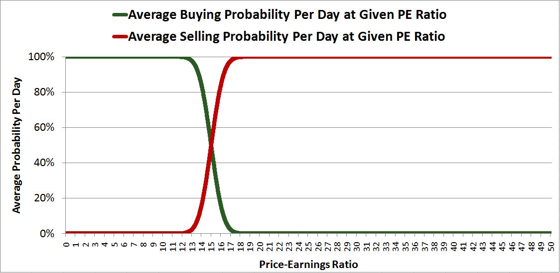
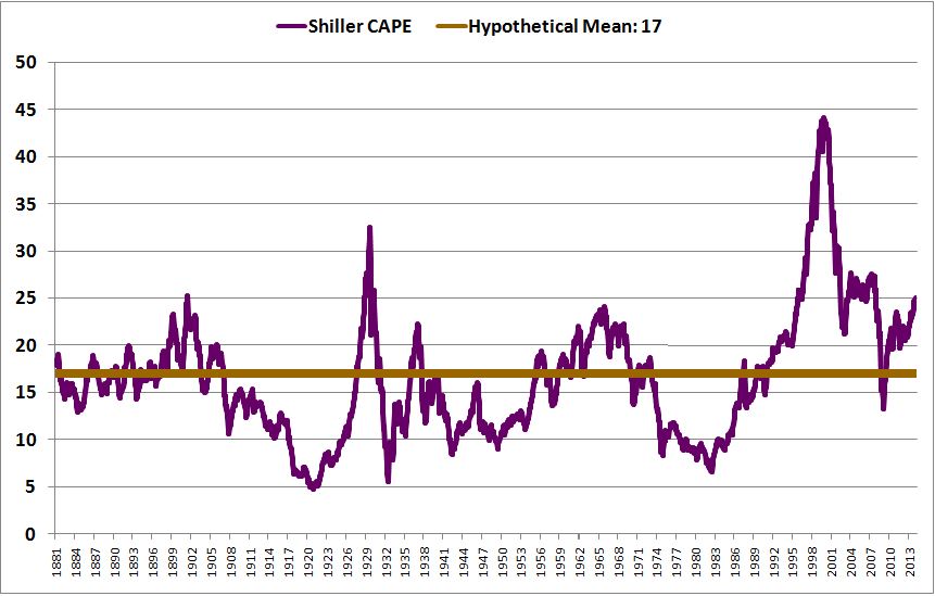
We’ve centered the functions around a PE ratio of 15, which we’ll assume is the “normal” PE, the PE that market participants are trained and accustomed to view as “fair.”  Per the above construction of the function, at a PE 15, there is a 50% chance per day that a given dollar in the system will be submitted to the market by a buyer to purchase stock, and a 50% chance per day that a given dollar’s worth of stock in the system will be submitted to the market by a seller to purchase cash (what selling is, inversely).  As the PE rises above 15, the buying probability falls sharply, and the selling probability rises sharpy.  As the PE falls below 15, the buying probability rises sharply, and the selling probability falls sharply. Evidently, the buyers and sellers are extremely price and valuation sensitive.  15 plus or minus a point or two is the range of PE they are willing to tolerate; whenever that range is breached in the unattractive direction, they quickly step away.

Now, if we wanted to make the function more accurate and realistic, we would make it a function not only of price and earnings, but also of interest rates, demographics, growth outlook, culture, past experience, and so on–all of the “variables” that conceivably influence the valuations at which valuation-sensitive buyers and sellers are likely to buy and sell.  We’re ignoring these factors to keep the problem simple.

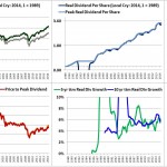
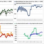
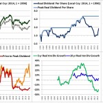
In the first instance, let’s assume that the supply of cash stays constant and the earnings stay constant.  Starting with a price of 2,000 for the index, holding the number of shares constant, and iterating through to an equilibrium, we get a chart that shows the trajectory of price over time, from now, the year 2014, to the year 2028.

noepsgnocashg

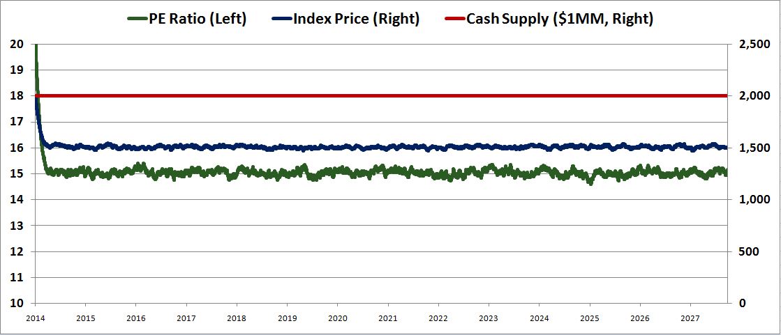
The result is as expected.  If the buyers are highly value sensitive, and if the earnings aren’t growing, then the price should settle tightly on the price range that corresponds to a “normal” PE ratio–in this case, a range around 1500, 15 times earnings, which is what we see.

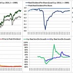
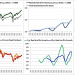
Now, let’s run the simulation on the assumption that the supply of cash stays constant and the earnings grow at 10% per year.

epsgnocashg

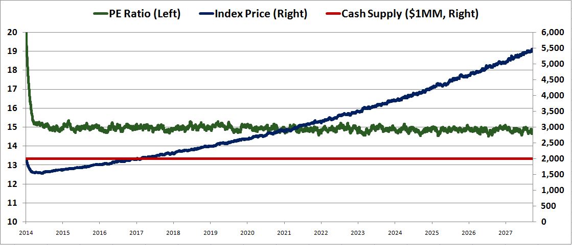
The result is again as expected.  The index price, the blue line, initially falls from 2000 to 1500 to get from a PE ratio of 20 to the normal PE ratio of 15.  It then proceeds to grow by 10% per year, commensurately with the earnings.  The cash supply stays constant, but this doesn’t appreciably hold back the price growth, because the buyers are value sensitive. They are going to push the price up to ensure that the PE ratio stays around 15, no matter the supply.

If you look closely, you will notice that the green line, the PE ratio, drifts slightly below 15 as time passes.  This drift is driven by the stunted supply effect.  The quantity of cash is not growing, which holds back the price growth by a miniscule amount relative to what it would be on the assumption of a perfectly constant 15 PE ratio.  The supply effect in the scenario is tiny, but it’s not exactly zero.

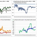
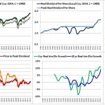
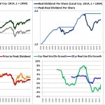
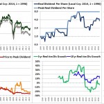
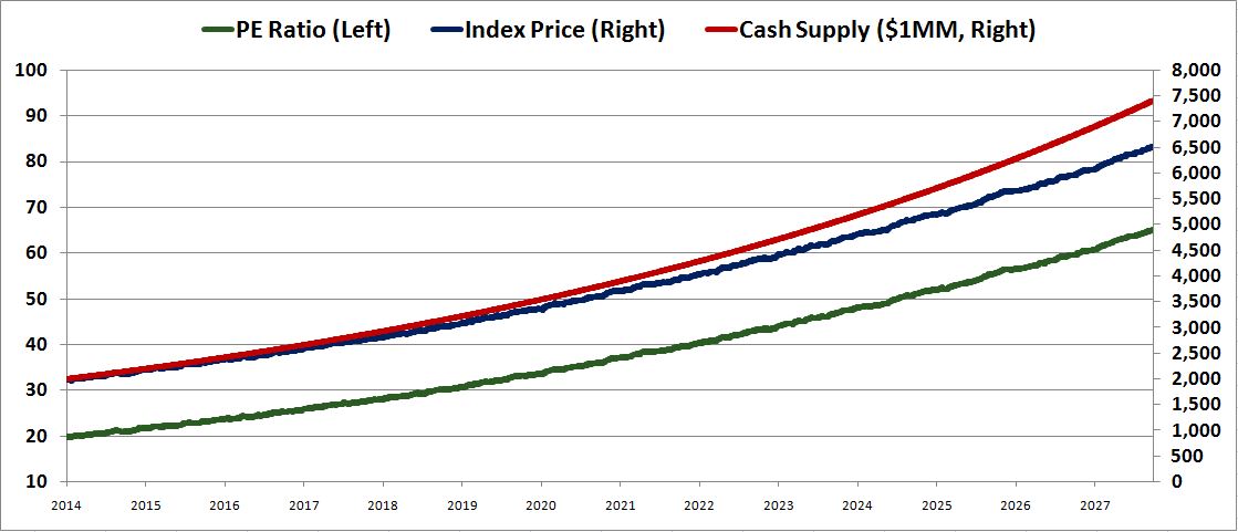
Now, let’s run the simulation on the assumption that the supply of cash rises at 10%, but the earnings stay constant.

cashgnoepsg

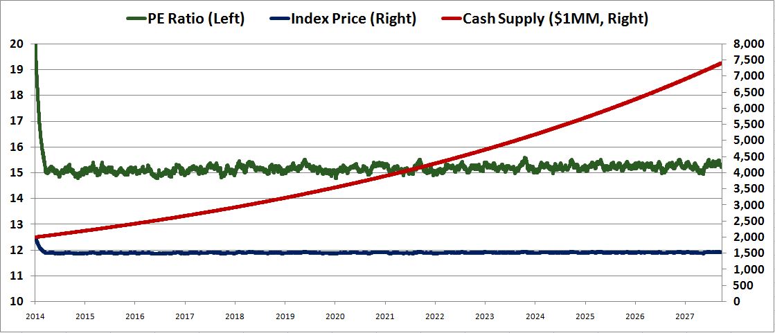
The result is again as expected.  The index price stays constant, on par with the earnings, which are not growing.  The cash supply explodes, but this doesn’t exert an appreciable effect on the price, because the buyers are extremely value sensitive.

If you again look closely, you will notice that the green line, the PE ratio, drifts slightly above 15 as time passes.  This drift is again driven by the stunted supply effect.  The quantity of cash is growing rapidly, and this pushes up the price growth by a miniscule amount relative to what it would be on the assumption of a perfectly constant 15 PE ratio.

Now, let’s introduce a buy-sell probability function that is minimally sensitive to valuation, and see how the system responds to supply changes.  Instead of using CDFs of Gaussian distributions with very small standard deviations, we will now use CDFs of Gaussian distributions with very large standard deviations.  In the actual simulations, we will also insert larger random deviations and offsets to help further model the price insensitivity.

novalsens

Evidently, under these new functions, the buying and selling probabilities remain essentially stuck around 50%, regardless of the PE ratio.  The functions are only minimally negatively-sloping and positively-sloping.  What this means qualitatively is that buyers and sellers don’t care much about the PE ratio, or any other factor related to price.  Price is not a critical consideration in their investment decision-making process.  They will accept whatever price they can get in order to take on or avoid the desired or unwanted exposure.

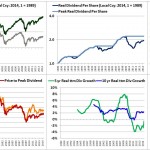
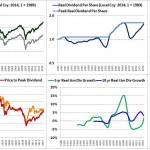
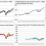
Now, let’s run the simulation on the assumption that the cash supply grows at 10%, while the earnings stay constant.

cashgrow

Here, the outcome changes significantly.  The index price, shown in blue, separates from the earnings, and instead tracks with the growing cash supply, shown in red.  Instead of holding at 15, the PE ratio, shown in green, steadily expands, from 20 in 2014 to roughly 65 in 2028.  All of the market’s “growth” ends up being the result of multiple expansion driven by the growth in the cash supply–growth in the amount of cash “chasing” the limited amount of shares.  Now, there is still some valuation sensitivity, which is why the index price fails to fully keep up with the rising cash supply.  The valuation sensitivity acts as a slight headwind.

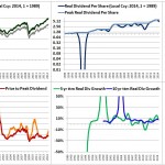
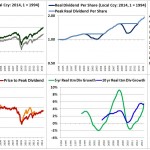
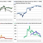
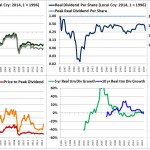
Now, let’s run the simulation on the assumption that the earnings grow at 10%, but the cash supply shrinks by 10%.

cashshrink

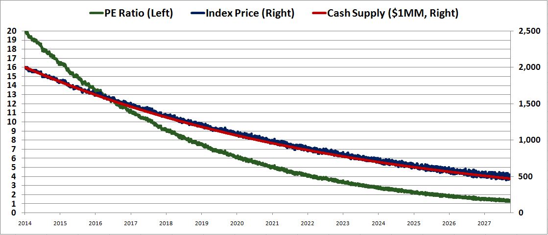
Once again, the price tracks with the contracting supply of cash, not with the growing earnings.  Consequently, the PE ratio falls dramatically–from 20 down to 1.25.

Supply Manipulations in a Live Experiment

Everything that we’ve presented so far is theoretical.  We don’t have a buy-sell probability function for real buyers and sellers that we could use to determine the prices that their behaviors will produce in a market with a growing supply of cash and fluctuating earnings. Even if we could come up with such a function, it would not be useful for making actual price predictions, as it would contain far too many fuzzy and hard-to-measure variables, and would always be changing in unpredictable ways.

At the same time, the modeling that we’re doing here is useful in that it allows us to think more clearly about the way that supply factors interact with buying and selling probability factors to determine price.  When confronted with questions about the impact of supply factors in specific market circumstances, the best approach to evaluating these questions is to explore the kinds of buying and selling probabilities that those circumstances will lend themselves to–that is, the kind of buy-sell probability functions the circumstances will tend to produce.

If the circumstances will tend to produce significant price and value sensitivity–that is, sharply negatively-sloping buying probabilities and sharply positively-sloping selling probabilities, as a function of price–then supply will not turn out to be a very important or powerful factor in determining price.  As supply differences lead to price changes, the number of people that want to buy and sell at the given price will quickly adjust, arresting the price changes and stabilizing the price.

But if the circumstances will tend to lend themselves to price and valuation insensitivity–that is, flatly-sloping buying and selling probabilities, or worse, reflexive buying and selling probabilities, buying probabilities that rise with rising prices, and selling probabilities that rise with falling prices–then supply as a factor will prove to be very important and very powerful.  As supply differences emerge and cause price changes, the number of people that want to buy and sell at the given price will not adjust as needed, causing the price to continue to move, the momentum to continue to carry.

With this in mind, let’s qualitatively examine a famous genre of experiments that economists have performed to test the impact of supply on price.  In these experiments, a large closed group of market participants are endowed with a portfolio of cash or stock, and are then left to trade the cash and stock with each other.

price

The shares of stock pay out a set quantity of dividends on a scheduled periodicity throughout the scenario, or at the end, and then they expire worthless.  Each dividend payment equals some constant value, plus a small offset that is randomly computed in each payment period.

At any time, it’s easy to calculate what the intrinsic value of a share is.  It’s the sum of the expected future dividend payments up to maturity, which is just the number of dividend payments that are still left to be paid, times the value of each payment.  The offset to the payments is random, it acts in both directions, therefore it effectively drops out of the analysis.  Granted, the offsets insert an “uncertainty” into the value of the shares, the undesirability of which investors might choose to discount.  But the uncertainty is small, and the participants aren’t that sophisticated.

Before the experiment begins, the experimenters teach the participants how to calculate the intrinsic value of a share.  The experimenters then open the market, and allow the participants to trade the assets with each other (through a computer).  Crucially, whatever amount of money the participants end up with at the end of the experiment, they get to keep.  So there is a financial incentive to trade and invest intelligently, not be stupid.

The experiment has been run over and over again by independent experimenters, incorporating a number of different individual “tweaks.”  It’s been run on large groups, small groups, financially-trained individuals, non-financially-trained individuals, over short time periods, long time periods, with margin-buying, without margin-buying, with short-selling, without short-selling, and so on.

The experiments consistently produce results that defy fundamentals, results in which prices deviate sharply from fair value, when in theory they shouldn’t.  Shown below is a particularly egregious example of the deviation, taken from an experiment run on 304 economic students at Indiana University consisting of a 15 round trading period that lasted 8 weeks:

expectediv

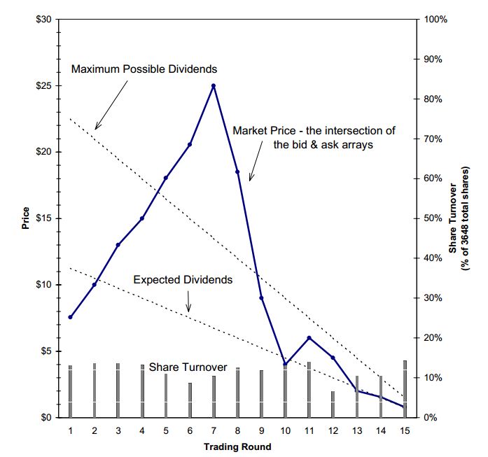
As you can see, the price deviates sharply from intrinsic value.  In the early phases, the buyers lack courage to step up and buy, so the price opens below fair value.  As the price rises, the buyers gain confidence, and more and more try to jump on board.  This process doesn’t stop when the limits of fair value are reached; it keeps going.  Buyers throw caution to the wind, and push the market into a bubble.  The bubble then bursts.  As the maturity nears, the price gravitates back towards intrinsic value.

If we think about the experiment, it’s understandable that this outcome would occur, at least in certain circumstances. “As long as the music is playing, you have to get up and dance.” Right?  Valuation is important only to the extent that it impacts price on the time horizons that investors are focused on.  In the beginning of the experiment, the investors are not thinking about what will happen at the end of the experiment, which is many months away.  They are thinking about what price they will be able to sell the security for in the near term.  They want to make money in the near-term, do what the other successful people in the game seem to be doing.  As they watch the price travel upward, above fair value, they start to doubt whether valuation is something that they should be focusing on. They conclude that valuation doesn’t “work”, that it’s a red herring, that focusing on it isn’t the way you’re supposed to play the game.  So they set it aside, and focus on trying to profit from the continued momentum instead.  In this way, they contribute to the growing excesses, and help create the eventual bubble.

As the security gets closer to its maturity, more and more participants start worrying about valuation.  It can’t be ignored forever, after all, for the bill’s eventually going to come due. And so as the experiment draws to a close, the price falls back to fair value.

Now, the question that we want to ask is, if we change the aggregate supply of cash in this experiment relative to the supply of shares, what will happen?  Of course, we already know the answer.  The valuation excesses will grow, multiply, inflate.  The buyers, after all, have demonstrated that they are not value sensitive–if they were, they wouldn’t let the price leave the fair value range.  As the price rises in response to the supply imbalances, the buyers aren’t going to pull back, and the sellers aren’t going to come forward–therefore, the imbalances aren’t going get relieved.  The price will keep rising until something happens to shift the psychology.

Interestingly, one practical finding from the experiment is that the most effective way to arrest the excess is to reduce the supply of cash relative to the supply of shares. When you reduce the supply of cash, the bubbles have a much more difficult time forming and gaining traction.  Sometimes, they don’t form at all.  Central Banks of the world, take note!

Now, some have objected to the results of the experiments, arguing that the participants often don’t understand how the maturity process works–that they often don’t recognize, until late in the game, that the security is going to expire worthless.  Put differently, the participants wrongly envision the dividends as investment returns on a perpetual security, rather than as returns of capital on a decaying security.  For our purposes, this potential flaw in the experiment doesn’t really matter, for even if the value of the security is misunderstood, that alone shouldn’t cause supply changes to appreciably impact prices. Supply should only appreciably impact prices if investors are not paying attention to value. Evidently, they aren’t.

A potentially more robust version of the experiment is one where there are no interim dividends, but only a single final payment, a single return of capital, paid to whoever owns the shares at the end.  In this version of the experiment, it’s painfully obvious what the security is worth, there is no room for confusion.  The security is worth the expected value of the final payment.

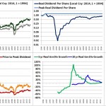
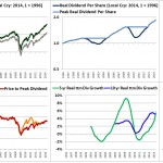
Professor Gunduz Caginalp of the University of Pittsburgh ran the experiment under this configuration, allowing groups of participants to trade cash and shares that pay an expected value of $3.60 at maturity (the actual value has a 25% chance of being $2.60, a 25% chance of being $4.60, and a 50% of being $3.60).  In one version, he kept the supply of cash roughly equal to the supply of shares, in another version, he roughly doubled the supply of cash.  He then ran each version of the experiment multiple times on different groups of participants to see whether the different versions of the experiment produced different prices.  The following chart shows the average price evolution for each version:

cashshars

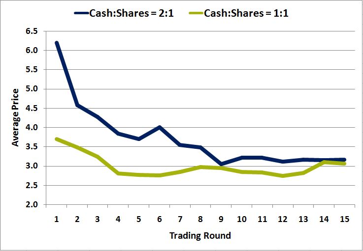
As you can see, the version in which the supply of cash is twice the supply of shares (blue line) produces prices that are persistently higher than the version in which the supply of cash equals the supply of shares.  This is especially true in the early trading rounds of the experiment–as the experiment draws to an end, valuation sensitivity increases, and the average prices of the two versions converge.

Interestingly, in the later rounds, the market in the high cash scenario seems to have an easier time moving the price to fair value than in the low cash scenario.  In the low cash scenario, a meaningful discount to fair value remains right up until the last few rounds, a discount that defies fundamental justification (why should the price be roughly $2.75 in round 12 when there is a 75% change of the price being substantially higher, and essentially a 0% chance of the price being lower, at maturity?).  This peculiarity illustrates the previous point that even when valuation is the dominant consideration for market participants, even when the market in aggregate is trying to move the price to fair value, supply still matters–it can nudge the market in the right or wrong direction.

It turns out that the only consistently reliable way to prevent an outcome in which individuals push prices in the experiment out of the range of fair value is to run the experiment on the same subjects multiple times–then, the investors learn their lessons. They start paying attention to valuation.

Evidently, the perceived connection between valuation and investment returns–the connection that leads investors to care about value, and to use it in their investment processes–is learned through experience, at least partially.  To reliably respect valuation, investors often need to go through the experience of not respecting it, buying too high, and then getting burned.  They need to lose money.  Then, valuation will become important, something to worry about.  Either that, or investors need to go through the experience of buying at attractive prices and doing well, making money, being rewarded.  In response to the supportive feedback, investors will grow hungry for more value, more rewards.

As with all rules that investors end up following, when it comes to the rule “though shalt respect value”, the reinforcement of punishment and reward, in actual lived or observed experience, cements the rule in the mind, and conditions investors to obey it.

Posted in Uncategorized | Comments Off on Supply and Demand: Untangling the Market’s Greatest Mystery

Why is the Shiller CAPE So High?

Why is the Shiller CAPE so high?  In the last several weeks, a number of prominent academics and financial market commentators have attempted to answer this question, to include the inventor of the valuation measure himself, Nobel Laureate Robert Shiller.  In this piece, I’m going to attempt to give a clear answer.

The piece has five parts:

  • In the first part, I’m going to explain why valuations in general are higher than they have been historically.  It’s not just the CAPE that’s historically elevated; the simple TTM P/E ratio is also historically elevated, by a reasonably large amount.
  • In the second part, I’m going to highlight the main reason that the Shiller CAPE has risen relative to the simple TTM P/E over the last two decades: high real EPS growth. I’m going to introduce a schematic that intuitively illustrates why high real EPS growth produces a high Shiller CAPE.
  • In the third part, I’m going to explain how reductions in the dividend payout ratio have contributed to high real EPS growth.  In discussing the dividend payout ratio, I’m going to present a different, potentially more accurate formulation of the Shiller CAPE, a formulation that conducts the calculation based on total return instead of price.  On this formulation, the Shiller CAPE falls by around 10%, from 26.0 to 23.5.
  • In the fourth part, I’m going to explain how a secular uptrend in profit margins has contributed to high real EPS growth over the last two decades.  This effect is the most powerful of all, and is the main reason why the Shiller CAPE and the TTM P/E have diverged in their valuation signals.
  • In the fifth part, I’m going to outline a set of possible future return scenarios that investors at current valuations can reasonably expect.  I’m then going to identify the future return scenario that I find most credible.

Higher P/E Valuations Generally

It’s important to note at the outset that the Shiller CAPE isn’t the only price-to-earnings (P/E) metric that is currently elevated. The good-old-fashioned trailing twelve month (TTM) P/E ratio is also elevated. With the index at 2000 and 2Q TTM reported earnings per share (EPS) at 103.5, the current TTM P/E is 19.3 (the number doesn’t change much if we use use TTM operating earnings, since the economy is in expansion, and writedowns are no longer a big impact). The historical average for the TTM P/E is 14.6. So, on a simple TTM P/E basis, the market is already 33% above its historical average.

Note that I did not say that the market is 33% “overvalued”–to call the market “overvalued” would be to suggest that it shouldn’t be at the valuation that it’s at.  This is too strong.  Not only is it possible that the market should be at its current valuation, it’s also possible that the market should be at a still higher valuation, and that it’s headed to such a valuation.

Now, to the crucial point that market moralists consistently miss.  The market’s valuation does not arise out of the application of any external standard for what “should” be the case. Rather, the market’s valuation arises as an inadvertent byproduct of the equilibriation of supply and demand: the process through which the quantity of equity being supplied by sellers achieves an equilibrium with the quantity of equity being demanded by buyers.  In a liquid market, the demand for equity must equal the supply on offer.  “Price” is the factor that changes so as to cause the two to equal.  In a normal, well-anchored market, higher prices lead to reduced demand and increased supply on offer, and lower prices lead to increased demand and reduced supply on offer.  If, at a given market price, the demand for equity exceeds the supply on offer, the market price will rise, which will lower the demand and increase the supply on offer, pulling the two back into equilibrium. Similarly, if, at a given market price, the demand for equity falls short of the supply on offer, the market price will fall, which will increase the demand and reduce the supply on offer, again pulling the two back into equilibrium.

Right now, the price necessary to bring the demand for equity into equilibrium with the supply on offer happens to be higher, relative to earnings, than the price that successfully achieved the same equilibrium in the past.  In a prior piece, I laid out a number of possible reasons for this shift.  The most important reason has to do with expectations about future interest rates. Right now, the market’s expectation is that future interest rates will be low–less than 2%, on average–for the next several decades, and maybe for the rest of time.

The interesting thing about markets is that investors in aggregate have to hold every asset in existence, including what is undesirable–in this case, low-return cash and fixed income. Obviously, investors are not going to want to hold low-return cash and fixed income in lieu of equities unless they expect that: (1) equities at current prices will also offer low future returns on the relevant long-term horizons, or (2) catalysts will emerge that will lead other investors to focus on the short-term and sell, leaving behind painful mark-to-market losses that those who are stuck in the market will have to endure, and, conversely, affording exciting “buying opportunities” that those who are out of the market will get to capitalize on.

We are at a point in the economic cycle where the fear of (2) on the part of those invested, and the hope for (2) on the part of those on the sidelines, is fading.  As the economy strengthens in the presence of highly supportive Fed policy–policy that everyone knows will remain supportive for as far as the eye can see–those that are invested in the market are becoming less and less afraid of corrections, and those on the sidelines are growing more and more frustrated waiting in vain for them to happen.  Crucially, those on the sidelines sense the growing confidence levels of their fellow investors, and are increasingly resigning themselves to the fact that the kinds of catalysts that might break that confidence, and produce meaningfully lower prices, are unlikely to emerge in the near term.  Consequently, the market is slowly and painfully being pushed upward into the first condition, a condition where equity valuations rise until investors become sufficiently disenchanted with them that they willingly settle for holding low return cash and fixed income instead–not briefly, in anticipation of a correction that is about to happen, but for the long haul.

Some would say that market prices have gone too far, and that equities are now offering no excess return relative to cash and fixed income–or even worse, a negative excess return.   But those that reach this conclusion are estimating long-term equity returns using a method that makes aggressive assumptions about the trajectory of future profit margins, assumptions that will probably prove to be incorrect, if recent experience is any indication of what’s coming.

Real EPS Growth: Impact on the Shiller CAPE

Returning to the Shiller CAPE, its current value is 26.0.  Its long-term historical average (geometric) is 15.3.  On a Shiller CAPE basis, the market is 70% above its long-term historical average.  It follows that almost half of the Shiller CAPE’s current elevation, 33% out of the overall 70%, can be attributed to the elevation of the simple TTM P/E measure.

This fact usually gets missed in discussions about the CAPE because market participants tend to analyze the market’s valuation in terms of forward earnings estimates.  On the most recent estimates for year-end 2015, the market’s P/E is 15.1, a number almost perfectly in-line with the historical average.  But this number is pure fantasy.

dfjkela

For the number to actually be achieved, the S&P will need to generate $132.30 in reported earnings for 2015–a growth of almost 30% over the next 16 months, off of earnings and profit margins that are already starting at extreme highs.  How exactly will this supergrowth be achieved?  Will S&P 500 revenues–and the overall U.S. GDP which they track–see 30% nominal growth over the next year and a half?  Are profit margins going to rise by 30%, from 10% to 13%?  Macroeconomically, the estimate makes no sense.

Now, let’s compare the valuation signal of the Shiller CAPE to the valuation signal of the simple TTM P/E across history.  The following chart shows the percent difference between the CAPE valuation signal (the ratio of the CAPE to its historical average) and the TTM P/E valuation signal (the ratio of the TTM P/E to its historical average) from 1881 to 2014:

diffgge

When the blue line is positive, the CAPE is calling the market more expensive than the TTM P/E.  When the blue line is negative, the CAPE is calling the market cheaper than the TTM P/E.  Right now, the CAPE is calling the market more expensive than the TTM P/E, but not by an extreme amount–the difference between the two metrics is in-line with the difference seen during other periods of history.

With the exception of the large writedown-driven gyrations of the last two recessions, you can see that over the last two decades, the CAPE has consistently called the market more expensive than the TTM P/E.  But that hasn’t always been the case.  For much the 1980s and early 1990s, the tables were turned; the CAPE depicted the market as being cheaper than the TTM P/E.

Now, why does the CAPE sometimes depict the market as more expensive than the ttm P/E, and sometimes cheaper?  The main reason has to do with the rate of real EPS growth over the trailing ten year period.  Recall that the Shiller CAPE is calculated by dividing the current real price of the index by the average of each month’s real TTM EPS going back 10 years (or 120 months).  When the real TTM EPS has grown significantly over the trailing 10 year period, this average tends to deviate by a larger amount from the most recent value, the value that is used to calculate the TTM P/E.

The point can be confusing, so I’ve attempted to concretely illustrate it with the following schematic:

akleja

Consider the high real growth scenario on the left.  Real EPS grows from $100 to $200 over a ten year period.  The average of real EPS comes out to $150, relative to the most recent real TTM EPS number of $200.  The difference between the two, which drives the difference between the valuation signals of the CAPE and the TTM P/E, is high, around 33%.

Now, consider the low real growth scenario on the right.  Real EPS grows from $100 to $110 over a ten year period.  The average of real EPS comes out to $105, relative to the most recent real TTM EPS number of $110.  The difference between the two, which drives the difference between the valuation signals of the CAPE and the TTM P/E, is low, around 5%.

As you can see, on a Shiller CAPE basis, the market ends up looking much cheaper in the low real growth scenario than in the high real growth scenario, even though the valuation is the same on a TTM basis.  This result is not in itself a mistake–the purpose of the CAPE is to discount abnormal EPS growth that is at risk of being unwound going forward.

To further confirm the relationship, consider the following chart, which shows the percent difference between the valuation signals of the CAPE and TTM P/E (blue) alongside the real EPS growth rate of the prior 10 years (red):

diffbtCAPETTM

As expected, the two lines track very well.  In periods of high real EPS growth, the market ends up looking more expensive on the CAPE than on the TTM P/E.  In periods of negative real EPS growth, the market ends up looking less expensive on the CAPE than on the TTM P/E.

Over the last two decades, the S&P 500 has seen very high real EPS growth–6% annualized from 1992 until today.  For perspective, the average annual real EPS growth over the prior century, from 1871 to 1992, was only 1%.  This rapid growth, along with changes to goodwill accounting standards that severely depressed reported earnings during and after the last two recessions (the latter of which is now out of the trailing ten year average, and no longer affecting the CAPE), explains why the CAPE has been high relative to the TTM P/E.

But why has real EPS growth been so high over the last two decades?  Before we explore the reasons, let’s appraise the situation with a simple chart of real TTM reported EPS for the S&P 500 from 1962 to present, with the period circa 1992 circled in red:

real ttm eps

Surprisingly, from 1962 to 1992, real TTM EPS growth was zero.  For literally 30 years, the S&P produced no real fundamental return, outside of the dividends that it paid out. But since then, real EPS growth has boomed.  From 1992 until 2014, S&P earnings have quadrupled in real terms.  Why has real EPS growth picked up so much in the last two decades?  There are two main reasons, which we will now address.

Changes in the Dividend Payout Ratio

The first reason, which is less impactful, has to do with changes in the dividend payout ratio.  Recall from a prior piece that dividends and growth are fungible.  If the corporate sector lowers its dividend payout ratio to fund increased internal reinvestment (capex, M&A, buybacks), real EPS growth will rise.  If it lowers its internal reinvestment (capex, M&A, buybacks) to fund an increase in dividends, real EPS growth will fall.  Assuming that the market is priced at fair value, and that the return on equity stays constant over time, the effects of the change will cancel, so that shareholders end up with the same return.

The chart below, from a prior piece, illustrates the phenomenon.  Over the long-term, the real return contribution from dividends (green) can rise or fall, but it doesn’t matter–the return contribution from real EPS growth (gold) shifts to offset the change, and keep the overall shareholder return constant (historically around 6%, assuming prices start out at fair value).

70yr Trailing 6%

Now, we know that the dividend payout ratio for US equities has fallen steadily since the late 19th century, and therefore we should expect real EPS growth now to be higher than in the past.  The following chart shows the trailing 10 year average dividend payout ratio for the S&P 500, from 1881 to 2014:

dkhs

But how much of a difference does the change in the dividend payout ratio make, as far real EPS growth and the Shiller CAPE are concerned?  The question is hard to answer. One thing we can do to get an idea of the size of the difference is to build a CAPE using a total return index instead of a price index.  Using a total return index instead of a price index puts all dividend payout ratios on the same footing.

The following chart shows the Shiller CAPE constructed using a total return index (blue) instead of a price index (red), from 1891 to 2014:

spx shillerdivp

[Details: The Total Return Shiller CAPE is constructed as follows.  Start with 1 share of the S&P 500 at the beginning of the data set.  Reinvest the dividends earned by that share, and each subsequent share, as they are paid out.  The result will be an index of share count that grows over time.  To calculate the Total Return Shiller CAPE, take the current real price times the current number of shares, and divide that product by the average of the real price times the number of shares that were owned in each month, going back 10 years or 120 months.  Then normalize the result for apples-to-apples numeric comparison with the original Shiller CAPE.]

[Note: The flaw in this measure is that it quietly rewards markets that are overvalued and quietly punishes markets that are undervalued.  The dividend reinvestment in overvalued markets gets conducted at less accretive prices than the dividend reinvestment in undervalued markets, causing the metric to shift slightly in the lower direction for overvalued markets, and slightly in the upward direction for undervalued markets.  To address this problem, we could hypothetically conduct the dividend reinvestments at “fair value” instead of at the prevailing market price–but we don’t yet have an agreed-upon way of measuring fair value!  We’re trying to build such a measure–a measure that appropriately reflects the impact of dividend payout ratio changes.]

With the S&P at its current level of 2000, the Total Return Shiller CAPE comes in at around 23.5, 10% below the original Shiller CAPE, which is currently at 26.0.  A 10% difference isn’t huge, but it still matters.

Changes in the Profit Margin

The bigger factor underlying the strong growth in real EPS over the last two decades, and the associated upward shift in the Shiller CAPE relative to the TTM P/E, has been the trend of increasing profit margins, a trend that began in 1992, and that continues intact to this day.  To understand the powerful effect that changes in profit margins can have on real EPS growth, let’s take a moment to consider the drivers of aggregate corporate EPS growth in general.

There are three ways that the corporate sector can grow its EPS in aggregate:

  • Inflation: The corporate sector can continue to make and sell the same quantity of things, but sell them at higher prices.  If profit margins remain constant, then the growth will translate entirely into inflation.  There will not be any real income growth of any kind–no real EPS growth, no real sales growth, no real wage growth–because the price index will have shifted by the same nominal amount as each type of income.
  • Real Sales Growth: The corporate sector can make and sell a larger quantity of things at the same price.  If profit margins remain constant, the result will be real growth in each type of income: real EPS growth, real sales growth, and real wage growth.  Each type of income will rise proportionately amid a constant price index, allowing the lot of every sector of the economy to improve in a real, sustainable manner.
  • Profit Margin Shift: The corporate sector can make and sell the same quantity of things at the same price, but then claim a larger share of the income earned from the sale. The shift will show up entirely as real EPS growth, but with no real sales growth, and negative real wage growth–“zero-sum” growth for the larger economy.

[Note: the corporate sector can also grow its nominal EPS by shrinking its outstanding share count through M&A and share buybacks.  But this “float shrink” needs to be funded.  If it is funded with money that would otherwise have gone to dividends, then we’re back to the fungibility point discussed earlier–on net, shareholders will not benefit.  If it is funded from money that would otherwise go to capex, then the effects of the reduction in share count will be offset by lower real earnings growth, and shareholders again will be left no better off.  If it is funded with an increased accumulation of debt–a “levering up” of corporate balance sheets–the assumption is that there will be a commensurate payback when the credit cycle turns, a payback in which dilutions, unfavorable financing agreements, and defaults undo the accretive effects of the prior share count reduction.  This story is precisely the one that unfolded from 2004 to 2008, and then from 2008 to 2010–a levered M&A and buyback boom significantly reduced the S&P share count, and then the dilutions of the ensuing recession brought the share count back to roughly where it began.]

In reality, aggregate corporate EPS tends to evolve based on a combination of all three processes occurring at the same time.  Some inflation, some real sales (output) growth, and some shift in the profit margin (cyclical or secular–either can occur, since profit margins are not a reliably mean-reverting series).  The important point to recognize, however, is this: real sales growth for the aggregate corporate sector (real increases in the actual quantity of wanted stuff that corporations make and sell, as opposed to inflationary growth driven by price increases) is hard to produce in large amounts, particularly on a per share, after-dilution basis.  For this reason, absent a profit margin change, it’s difficult for real EPS to grow rapidly over time.  Wherever rapid real EPS growth does occur, a profit margin increase is almost always the cause.

Not surprisingly, the real EPS quadrupling that began in 1992, and that that has caused the Shiller CAPE to substantially increase in value relative to the TTM P/E, has primarily been driven by the profit margin upshift that started in that year and that continues to this day.  In much the same way, the zero real EPS growth that investors suffered from 1962 to 1992, and that caused the market of the 1980s and early 1990s to look cheaper on a Shiller CAPE basis than on a TTM P/E basis, was driven primarily by the profit margin downshift that took place during the period.

The following chart shows the net profit margin of the S&P 500 on GAAP reported earnings from 1962 to 2014, with the period circa 1992 circled in red:

pmreal

The following chart superimposes real EPS (green) onto the profit margin (blue):

profmarginincluded

As you can see, profit margins began the period in 1962 at almost 7%, and bottomed in 1992 at less than 4%, leaving investors with zero real EPS growth over a period of roughly thirty years.  From 1992 until today, profit margins rose from 4% to 10%, leaving investors with annualized real EPS growth of 6%, more than three times the long-term historical average (1871-2014), 1.8%.

Valuation bears have been warning about “peak profit margins” for four years now (and warned about them in the last cycle as well).  But profit margins keep rising.  In this most recent quarter, they reached a new record high, on top of the record high of the previous quarter, on top of the record high of the quarter before that.  What’s going on?  When is this going to stop, and why?

Nobody knows the answer for sure–certainly not the valuation bears who have continually gotten the call wrong.  But even the valuation bulls will have to acknowledge that the profit margin uptrend seen over the last two decades can’t go on forever.  It will have to eventually peter out–probably sooner rather than later.  If and when that happens, real EPS growth will be limited to the contributions of real sales growth from reinvestment and float shrink from M&A and share buybacks.  Neither phenomenon is capable of producing the kind of rapid real EPS growth that the S&P has seen over the last two decades (especially not the M&A and buybacks, which are occurring at lofty prices), and therefore the rate of real EPS growth should moderate, and the divergence between the Shiller CAPE and the TTM P/E should narrow.

Valuation: A Contingent Approach

In a prior piece, I argued that profit margins are the epicenter of the valuation debate.  All of the non-cyclical valuation metrics that purport to show that the market is egregiously overvalued right now rely on aggressive assumptions about the future trajectory of profit margins, assumptions that probably aren’t going to come true.  You can add the Shiller CAPE to that list, since its abnormal elevation relative to the TTM P/E is tied to the increase in profit margins that has occurred since the early-to-mid 1990s.

When investors discuss valuation, they often approach the question as if there were an objective, determinate answer.  But there isn’t.  At best, valuation is a contingent judgement–a matter of probabilities and conditionalities: “if A, then B, then C, then the market is attractively valued”, “if X, then Y, then Z, then the market is unattractively valued.”  There are credible scenarios where the current market could end up producing low returns (and therefore be deemed “expensive” in hindsight), and credible scenarios where it could end up producing normal returns (and therefore be deemed “cheap” in hindsight, particularly relative to the alternatives).  It all depends on how the concrete facts of the future play out, particularly with respect to earnings growth and the market multiple.  That’s why it’s often best for investors to just go with the flow, and not fight trends based on tenuous fundamental analysis that will just as often prove to be wrong as prove to be right.

With respect to the market’s current valuation and likely future return, let’s dispassionately examine some of the possibilities:

Possibilty #1: Moderately Bullish Scenario

The increase in profit margins that we’ve seen from the mid 1990s until now is retained going forward.  The increase doesn’t continue, but it also doesn’t reverse.  On this scenario, the market’s return will be determined by the fate of the P/E multiple.

At 19.3 times reported TTM earnings, and 17.9 times operating TTM earnings, the market’s P/E multiple is clearly elevated on a historical basis. But it doesn’t immediately follow that the market will produce poor returns going forward, because the multiple might stay elevated.

The most likely scenario in which profit margins hold up is one where where the corporate sector continues to recycle its capital into M&A, share buybacks, and dividends, while shunning expansive investment.  Generally, expansive investment brings about increased inter-firm competition and increased strain on the labor supply, both of which exert downward pressure on profit margins.  In contrast, capital recycling that successfully displaces expansive investment tends to bring about reduced inter-firm competition and reduced strain on the labor supply, both of which exert upward pressure on profit margins. The latter point is especially true of M&A, which has the the exact opposite effect on competition as expansive investment.

In a low-growth, low-investment, high-profit-margin world, where incoming capital is preferentially recycled into competition-killing M&A and float-shrinking share repurchases, rather than deployed into the real economy, interest rates will probably stay low.  The frustrated “reach for yield” will remain intact, keeping the market’s P/E elevated (or even causing it to increase further).  If the market’s P/E stays elevated, there is no reason why the market can’t produce something close to a normal real return from current levels–a return on par with the 6% real (8% to 10% nominal) that the market has produced, on average, across its history.  Relative to the opportunities on offer in the cash and fixed income spaces, such a return would be extremely attractive.

Now, even if the current market–at a TTM P/E of 19.3 times reported earnings and 17.9 times operating earnings–is set to experience multiple contraction and lower-than-normal future returns, it doesn’t follow that the market’s current valuation is wrong.  The market should be priced to offer historically low returns, given the historically low returns that cash and fixed income assets are set to offer over the next several decades.  Indeed, if the market were not currently priced for historically low returns, then something would be wrong.  Investors would not be acting rationally, given what they (should) know about the future trajectory of monetary policy.

Possibility #2: Moderately Bearish Scenario

The increase in profit margins is not going to fully hold.  Some, but not all, of the profit margin gain will be given back.  On this assumption, it becomes harder to defend the market’s current valuation.

Importantly, sustained reductions in the profit margin–as opposed to a temporary drops associated with recession–tend to occur alongside rising sales growth.  In terms of the effect on EPS, rising sales growth will help to make up for some of the profit that will be lost.  However, almost half of all sales growth ends up being inflation–the result of price increases rather than real output increases.  With inflation comes lower returns in real terms (the only terms that matter), and also, crucially, a tighter Fed.  If the Fed gets tighter, a TTM P/E of 19.3 will be much harder to sustain.  The market will therefore have to fight two headwinds at the same time–slow EPS growth due to profit margin contraction and a return drag driven by multiple contraction.  Returns on such a scenario will likely be weak, at least in real terms.

But they need not be disastrously weak.  In a prior piece, I argued that returns might end up being 5% or 6% nominal, or 3% or 4% real.  Of course, that piece assumed a starting price for the S&P 500 of 1775.  Nine months later, the index is already at 2000.  The estimated returns have downshifted to 3% or 4% nominal, and 1% or 2% real.  Such returns offer almost no premium over the returns on offer in the much-safer fixed income world, and therefore, if any kind of profit margin contraction is coming, then the current market is probably pushing the boundaries of defensible valuation.

Possibility #3: Aggressively Bearish Scenario

Profit margins are going to fully revert to the pre-1990s average.  On this assumption, the market is obscenelyoutrageously expensive.  If, at a profit margin of 9% to 10%, EPS comes in at $103.5, and if profit margins are headed to the pre-1990s average of 5% or 6%, then the implication is that EPS is headed to around $55 (a number that will be adjusted upward in the presence of sales growth and inflation–but only as time passes).  Instead of a historically elevated TTM P/E of 19, the market would be sitting at a true, normalized TTM P/E of around 36.

Obviously, if margins and earnings were to suddenly come apart, such that the S&P at 2000 shifts from being valued at 19 times earnings to being valued at 36 times earnings, as opposed to the “15 times forward” that investors think they are buying into, prices would suffer a huge adjustment.  If the shift were to happen quickly, over a short number of months or quarters, the market would almost certainly crash.

But even if the shift were to happen very slowly, such that EPS simply stagnates in place, without falling precipitously, real returns over the next decade, and maybe even the next two or three decades, would still end up being very low–zero or even negative.  The profit margin contraction would eat away at real EPS growth, as it did from the 1960s until the 1990s.  Even nominal returns over various relevant horizons might end up being zero or negative.

Possibility #4: Aggressively Bullish Scenario

Profit margins are going to continue to increase.  Now, before you viscerally object, ask yourself: why can’t that happen?  Why can’t profit margins rise to 12% or 14% or even higher from here?  The thought might sound crazy, but how crazy would it have sounded if someone were to have predicted, in 1992, with profit margins at less than 4%, that twenty years later profit margins would be holding steady north of 10%, more than 200 basis points above the previous record high?

If profit margins are set to continue their upward increase, then the market might actually be cheap up here, and produce above average returns going forward.  The same is true if P/E multiples are set to continue their rise–a possibility that should not be immediately dismissed.  As always, the price of equity will be decided by the dynamics of supply and demand.  So long as we continue to live in a slow growth world aggressively backstopped by ultra-dovish Fed policy, a world where investors want and need a decent return, but can only get one in equities, there’s no reason why the market’s P/E multiple can’t get pushed higher, to numbers above 20, or even 25.  It certainly wouldn’t be the first time.

Going forward, all that is necessary for such an outcome to be achieved is for investors to experience a re-anchoring of their perceptions of what is “appropriate”–become more tolerant, less viscerally afraid, of those kinds of valuation levels.  If the present environment holds safely for a long enough period of time, such a re-anchoring will occur naturally, on its own. Indeed, it’s occurring right now, as we speak.  Three years ago, nobody would have been comfortable with the market at 2000, 19 times trailing earnings. People were acclimatized to 12,  or 13, or 14, as “reasonable” multiple, and were even seriously debating whether multiples below 10 were going to become the post-crisis “new normal.”  The psychology has obviously shifted since then, and could easily continue to shift.

As for me, I tend to lean towards option #2: a moderately bearish outcome.  I’m expecting weak long-term returns, with some profit margin contraction as labor supply tightens, and some multiple contraction as Fed policy gets more normal–but not a return to the historical averages.  Importantly, I don’t foresee a realization of the moderately bearish outcome any time soon.  It’s a ways away.

I expect the market to eventually get slammed, and pay back its valuation excesses, as happens in every business cycle.  If this occurs, it will occur in the next recession, which is when valuation excesses generally get paid back–not during expansionary periods, but during contractions.  The next recession is at least a few years away, maybe longer, and therefore it’s too early to get bearish.  Before sizeable recession becomes a significant risk, the current expansion will need to progress further, so that more real economic imbalances are built up (more misallocations in the deployment of the economy’s real labor and capital resources), excesses that provoke rising inflation, and that get pressured by the monetary policy tightening that occurs in response to it.  In the meantime, I expect the market to continue its frustrating and painful grind higher, albeit at a slower pace, offering only small pullbacks in response to temporary scares.  Those who are holding out for something “bigger” are unlikely to be rewarded any time soon.

Given the headwinds, I think the long-term total return–through the end of the current business cycle–will be around 1% to 2% real, 3% to 4% nominal.  Poor, but still better than the other options on the investment menu.  An investor’s best bet, in my view, would be to underweight U.S. equity markets in favor of more attractively priced alternatives in Europe, Japan, and the Emerging Markets.

(h/t to the must-follow Patrick O’Shaughnessy @millennial_inv of OSAM for his valuable help on this piece)

Posted in Uncategorized | Comments Off on Why is the Shiller CAPE So High?

Global Stock Market Valuation and Historical Real Returns Image Gallery

In this piece, I’m going to analyze the historical local currency real total returns of different stock markets around the world: 46 different large cap indices, 12 different small and mid (SMID) cap indices, and, for the U.S., 4 different style indices–growth, momentum, quality, and value.  For each index, I’m going to generate a chart that visually captures key trends and data points, shown below with the Hong Kong stock market as the example:

hk1971

Theoretical background, and instructions for how to read and interpret the charts, are provided in the paragraphs below.  The charts are presented at the end.

Dividend Decomposition

We can decompose–separate, conceptually split apart–equity total returns into two components:

  • Dividend Return: the return due to dividends paid out and reinvested.
  • Price Return: the return due to changes in the market price

We can further decompose price return into two components:

  • Growth: the return due to growth in some chosen fundamental
  • Valuation: the return due to changes in market valuation measured in terms of that fundamental

To measure fundamental growth, we can choose any “fundamental” that we want, as long as the metric that we use to measure the change in valuation employs that same fundamental.  So, for example, we can decompose the price return into: the return due to earnings growth and the return due to the change in the price to earnings multiple.  Alternatively, we can decompose the price return into: the return due to book value growth and the return due to the change in the price to book multiple.  And so on.  We cannot, however, decompose the price return into: the return due to earnings growth and the return due to the change in the price to book multiple.  On such a decomposition, we would be mixing incompatible bases.

To conduct the decompositions, we’re going to use dividends as the fundamental.  We’re therefore going to decompose the real returns of each market into three components: the real return due to dividends paid out and reinvested at market prices, the real return due to growth of dividends, and the real return due to the change in the price to dividend multiple–which is just the inverse of the dividend yield.  Notice the aforementioned consistency between the fundamental and the valuation measure: we’re measuring fundamental growth in terms of dividend growth and changes in valuation in terms of changes in the price to dividend ratio.

We need to conduct the analysis in real terms–with each country’s returns adjusted for inflation–because inflationary growth is worthless to investors, yet it’s a significant driver of nominal equity returns–often, the most significant driver of all.  If we don’t adjust the returns for inflation, then the performance of the stock markets of high-inflation countries such as Hungary will appear vastly superior to the performance of the stock markets of low-inflation countries such as Germany, even though the performance is not any better in real terms.

There are three reasons why we’re going to use dividends as the fundamental, rather than earnings.  First, dividends are more stable across the business cycle than earnings.  Second, the accounting practices used to measure earnings are not the same across different countries, different periods of history, or even different phases of the business cycle.  But dividends are dividends–unambiguous, concrete, indisputable.   Third, for international markets, historical dividend data is more readily available than historical earnings data. MSCI provides total return and price return indices for all countries that have investible stock markets (available here).  In providing those indices, MSCI provides the materials necessary to back-calculate dividends across history.  We’re going to use the MSCI indices, which generally go back to 1971, along with international CPI data (available here), to conduct the decompositons.

Note that the dividends that we back-calculate in this way will be somewhat different from what you might see in an ETF or from an official indexing source–such as S&P or FTSE. As expected, the back-calculated dividends tend to closely match the dividend data on MSCI’s fact sheets, but even that data is not perfectly consistent with other sources.  Take any discrepancies lightly–it’s the big picture that we’re focused on here.

Now, the obvious problem with decomposing returns using dividends as the fundamental is that anytime the dividend payout ratio–the share of earnings that corporations pay out to their shareholders in the form of dividends–changes in a lasting, secular manner, we’re going to get distorted results.  Unfortunately, there’s no way to avoid this problem–we just have to deal with it.

Fortunately, most countries have maintained relatively consistent dividend payout ratios across history.  The U.S. is the obvious exception–but even with the U.S., the ensuing distortion isn’t too large, because in the historical period that we’re going to focus on–the early 1970s until the present day–dividend payout ratios haven’t changed by all that much.  The big downshift in payout ratios happened earlier, as you can see in the chart below, which shows smoothed dividends divided by smoothed earnings for the S&P 500:

shillerpayout

Trailing Twelve Month Dividends and Peak Dividends

Like earnings, dividends are cyclical, though to a much lesser degree.  To smooth out their cyclicality, we’re going to conduct the price return decomposition using two different formulations of the dividend: first, the simple trailing twelve month (ttm) dividend, second, the peak dividend–the highest dividend paid out in any twelve month period at any time in the past.

The ttm dividend decomposition will separate the price return into ttm dividend growth and changes in the price to ttm dividend ratio. The peak dividend decomposition will separate the price return into peak dividend growth and changes in the price to peak dividend ratio.  Both decompositions will be presented in the charts so that the reader can compare them.

The best cases of hidden value are those where the ttm dividend yield is very low, but the peak dividend yield is very high.  A sharp divergence between the two suggests that the market is only taking into consideration the current dividend, which may be temporarily depressed, and is ignoring the past dividends that the corporate sector paid out–dividends that it may end up being able to pay out in the future, when the temporarily depressed conditions improve.

valuation

The chart to the left ranks the stock markets of the world in terms of peak dividend yield and ttm dividend yield as of June 30, 2014.  Looking at Greece in specific, on a simple ttm basis, the dividend yield at current prices is a paltry 2.41%–hardly a signal of value.  But if you look at the peak dividend yield, which uses the highest dividend in Greece’s history–the dividend paid in the ’06-’07 period–the dividend yield at current prices comes in at a whopping 23.35%.

Now, it may be the case that the performance that the Greek corporate sector exhibited in ’06-’07 does not accurately represent the performance it is likely to exhibit in the future, and that the long-term yield that Greece will offer at current prices will be significantly lower, even as conditions in  Greece improve.  But even if we assume that the long-term yield at current prices will be dramatically lower–say, 75% lower–that’s still a 6% yield, which is an excellent yield.

Familiar readers will note that the country’s that show up as cheap and expensive in terms of peak dividend yields also show up as cheap and expensive in Mebane Faber’s global CAPE analysis.  The two metrics are reasonably consistent in their signals, which is to be expected, given that they are reading the same valuation reality.  As a valuation metric, CAPE is admittedly superior to the peak dividend yield, but it’s also more costly–you have to use ten years to calculate it, which means that you lose 10 years from the analysis. For many of these countries–those that only have 20 or 30 years of history–10 years is a lot to lose.

The Goal of the Decomposition

So why are we doing this decomposition?  What’s the point?  The reason we do the decomposition is because it gives us a rough picture of how much of a given countries’ stock market performance has been driven by changes in valuation, and how much has been driven by fundamentals.  Changes in valuation are a fickle driver of long-term returns. If a country has outperformed because it has gone from cheap to expensive, or if it has underperformed because it has gone from expensive to cheap, then as investors we should want to go the other way–invest in the cheap country, and not invest in the expensive country.

But, crucially, if the country has outperformed because its corporate sector has exhibited consistently poor fundamental performance, then we don’t necessarily want to go the other way.  Warren Buffet reminds us that sound fundamental investing is not just about buying companies on the cheap, but about buying good companies on the cheap.  Bad companies on the cheap–value traps–are return killers.  This fact is just as true on the country level as it is on the individual stock level.

When we look at the data, we’re going to quickly notice that the corporate sectors of some countries have performed much better–produced substantially more fundamental growth for each unit of reinvestment that they’ve engaged in–than the corporate sectors of other countries.  This outperformance may have been the result of coincidental tailwinds that will not obtain going forward, and therefore extrapolating the outperformance into the future may prove to be a mistake.  But the outperformance may also be a sign of the inherent superiority of the corporate sectors of some countries relative to the corporate sectors of other countries.  If it is, then we should preferentially seek out the superior countries, and be willing to pay more to invest in them, and avoid the inferior countries, demand more to invest in them.  Valuation matters to returns, but it’s not the only thing that matters.

Countries with corporate sectors that invest inefficiently and excessively, and that don’t respect the rights and interests of their shareholders, don’t tend to produce strong returns, even when they are bought on the cheap.  Take the example of Russia–a country notorious for its corruption, corporate waste, poor governance, and disrespect for property rights. Since 1996, the Russian stock market has averaged an atrocious -5% annual real total return.  This disastrous performance was not the result of a high starting valuation–the dividend yield in 1996 was above 2%, higher than for the U.S.  Rather, the underpformance is a result of the fact that dividends haven’t grown by a single ruble in real terms since 1996, even though Russia hasn’t paid out very much in dividends along the way.  If the Russian corporate sector was earning profit and reinvesting that profit the entire time–a full 18 years–where did the profit go?  It certainly didn’t go to shareholders, as they have nothing to show for it.

On the other extreme, since 1996, the U.S. stock market has averaged a healthy 6% real total return.  This 6% has not been driven by any kind of irresponsible valuation expansion–in dividend terms, valuations were roughly the same in 1996 as they are today. Rather, it was the result of solid corporate performance.  The U.S. corporate sector produced a 2% annual real return from dividends paid out to shareholders, and an impressive 3.25% in annual real dividend growth.  Changes in the U.S. market’s valuation added an additional 0.75% annually to the real return, producing a real total return of 6%.

The Payout Ratio: Inevitable Messiness

Now, the picture we will get from the decomposition will be admittedly messy, for a number of reasons.  First, we aren’t incorporating the average dividend payout ratios of each country into the analysis, therefore we can’t assess the price to dividend ratio as a valuation signal.  Is a price to dividend ratio of 50–i.e., a dividend yield of 2%–high, and therefore expensive?  It may be for Austria, but not necessarily for Japan.  Not knowing the dividend payout ratio, all we can do is compare the country’s current valuation to its own history, on the assumption that dividend payout ratios haven’t changed in a long-term, secular manner (and, to be fair, they may have).

Moreover, because we don’t know the dividend payout ratio, we don’t know how much growth we should expect out of each country. Countries that are reinvesting a large share of their cash flows in lieu of paying out dividends should be producing large amounts of growth–those that are doing the opposite should not be.   Using the information currently available, we can’t necessarily tell the difference.

Most importantly, we don’t know what the factors are that have caused the corporate sectors of some countries to perform substantially better than others.  The factors could be cyclical, macroeconomic, demographic, era-specific, driven by differences in industry concentrations, investment efficiency, corporate governance, shareholder friendliness, unsustainable booms in productivity, and so on–we don’t know.  Therefore we can’t necessarily be confident in projecting the past superior performance out into the future.

Still, the picture we get will give us a minimally sufficient look at what’s going on.  It will tell us where things have been going well for shareholders in terms of the growth and dividends that have been produced for them, and where things have not been going well. That knowledge should be enough to get us started on the important task of figuring out where the corporate overachievers and the value traps might lie.

How to Interpret the Charts

Consider the following chart, which decomposes the performance of Ireland from January 1989 to June of 2014:

ireland1989

The bright yellow in the left column (0.17%) is the actual annual real total return for the period.  The green (-0.68%) and blue (5.90%) below that is the annual real return contribution from growth plus dividends–which, notice, is what the real return would have been if there had been no change in valuation (the third component of returns removed).  The green (-0.68%) uses a ttm dividend basis, and the blue (5.90%) uses a peak dividend basis.

The pink below that (2.36%) is the annual contribution to real returns from reinvested dividends over the period.  It is calculated by taking the difference between the annual real total return for the period and the annual real price return for the period.  Below that is the annual contribution of dividend growth (-3.02%, 3.75%) and change in valuation (0.85%, -5.73%), measured under each basis (green = ttm dividend basis, blue = peak dividend basis).  Below that is an internal checksum of sorts, in which the contribution of the valuation change is calculated by a wholely different method, to make sure that the analysis is roughly correct.  You can ignore it.

In terms of the graphs, the upper left graph is the real total return (green) and the real price return (gray).  The upper middle graph is ttm real dividends per share (dark blue) and historical peak real dividends per share (light blue).  The upper right graph is the historical yield using the ttm dividend (purple, with the yellow box above showing the ttm dividend yield as of June 2014, which is 1.67%) and the peak dividend (hot pink, with the yellow box abvoe showing the peak dividend yield as of June 2014, which is 9.26%).  To review, the peak dividend yield is what the yield would be at a given time if the dividend went back to what it was at the largest point in time up to that time–for Ireland, it’s very high, because the dividends that Ireland paid out in the last cycle were very high relative to Ireland’s current price, which is depressed–you can interpret this as a sign of cheapness for the Irish market).  The lower left graph is the Price to ttm Dividend ratio (orange) and Price to Peak Dividend ratio (red) ratio.  The lower middle graph is the 5 year (light green) and 10 year (bright blue) growth rates of the real ttm dividend.

The lower right graph is a running estimate of future 5, 7, and 10 year Shillerized real returns using the “real reversion” method laid out in a prior piece.  We calculate this estimate by discounting the market’s average real return to reflect a reversion from the present valuation to the average valuation.

Now, let me be fully up front with the reader.  Like all backward-looking return estimates that purport to fit with actual forward-looking results across history, this estimate involves cheating.  We are using information about the average return for the entire data set, past and future, and the average valuation for the entire data set, past and future, to estimate the future return from past moments in time.  From the perspective of those moments, the average of the entire data set includes information about the future that was not known then–therefore, in projecting a reversion to the average, our estimates are taking a peak at the future.  That is, they are cheating.

You’ll see that the method often nails it, with extremely high correlations with actual returns, well above 90%. But don’t take that to mean anything special. As I’ve emphasized elsewhere, these types of fits are very easy to build in hindsight, because you can effectively peak ahead at the actual results, and utilize now-determined information about the future that was not determined–or knowable in any way–at the time that the prediction would have needed to have been made.

I introduce the real reversion estimates into the chart not to make any sort of confident prediction about what the forward real return of any given market will actually be–such a prediction would require a look that goes much deeper than a backwards-looking curve fit that exploits cheating–but simply to give the reader an idea of when, in the market’s history, valuations were cheap and expensive relative to their averages for the period, and where they are now, relative to their historical averages.  The averages for the period in question may not end up being the averages of the future, and therefore they may not be relevant to the future.

The Charts With Associated Tables

Finally, to the charts.  What follows is a user-controlled slideshow of charts for different countries across different time periods of history.  If you click on any image, it will put you into that country’s part of the slideshow.

Before each chart, there’s a table, sorted by country name, that presents all of the results.  To view the table, simply click on it.  On the right side of each table, there’s a section on “non-equity growth”, which includes potentially relevant information on population growth, real GDP growth per capita, and real GDP growth over the period (source here).

Jan 1971 to Jun 2014: Developed Market Returns

Table:

7114

Slideshow:

Jan 1989 to Jun 2014: Developed and Emerging Market Returns

Table:

8914

Slideshow:

Jan 1989 to Jun 2014: US Growth, Momentum, Value, Quality

Table:

style


Slideshow:

Jan 1994 to Jun 2014: Developed, Emerging and Frontier Market Returns

Table:

9414

Slideshow:

Jan 1996 to Jun 2014: Developed and Emerging Market Small and Mid Caps

Table:

9614smid

Slideshow:

1996 to 2014: Czech Republic, Egypt, Hungary, Russia

Table:

leftovers

Slideshow:

Conclusion

After examining the data, here are my conclusions:

  • Europe, in particular the PIIGS, are very cheap relative to their own valuation histories and relative to the valuations of other countries.  On a ttm dividend basis, the returns due to growth have been poor, but that’s because dividends have crashed to almost nothing in response to the crisis.  If dividends eventually return to where they were prior to 2008–a big if, but one worth considering–the returns of the European periphery countries, and of European countries in general, should be very attractive.
  • Japan’s underperformance since 1989 has been due primarily to an egregiously high starting valuation.  But this excess has been entirely worked off, and Japan now offers a higher dividend yield than the U.S.  Japan’s corporate performance, however, remains something of a mystery.  It’s hard to quantify Japan’s dividend payout ratio, and to therefore get an estimate of how much dividend growth should have occurred from 1989 to today, because Japanese earnings are significantly understated due to excessive depreciation.  If the Japanese dividend payout ratio relative to true earnings has been low, which it probably has been, then Japanese ROEs have been poor.  The country owes its shareholders more growth for the amount that it has allegedly “reinvested.”  If growth by capital investment is not possible in Japan given the aging, shrinking population demographics, and weak consumer demand, then earnings should be deployed into dividends and share buybacks.  If Abenomics manages to stimulate this outcome, and promote an associated improvement in shareholder yield, then Japanese equities should produce strong returns going forward.
  • Australia and New Zealand are reasonably valued, with healthy dividend yields.  But the commodity-centric earnings and dividends that they generated in the last cycle may not be sustained going forward.
  • The US is expensive relative to its own history and relative to other countries.  It’s among the most expensive stock markets in the world.
  • Emerging Markets are generally cheap, but, macroeconomically, it’s difficult to project their performance over the last 20 to 30 years out into the future.  Interesting countries to look at on valuation include Brazil, Singapore, and Taiwan.  Korea and Turkey, in contrast, are hardly cheap on a dividend basis, and have not performed well in terms of the amount of dividend growth that they have generated.
  • Russia and China are, at a minimum, weird.  Both have exhibited extremely volatile markets over the last 18 years, with dividend fluctuations tracking the price fluctuations.  Russia, in particular, has generated no real dividend growth since 1996, and also no real dividend growth since 2003, after the default.  Both markets are presently very cheap, but they won’t make for good investments unless they cease to be the value traps that they’ve proven themselves to be in the past.
  • For styles, counterintuitively, the “value” sector of the U.S. market is expensive, and the “quality” sector is cheap.  So if you’re looking to invest in the U.S., you’re best bet is probably to buy high quality multinationals with strong competitive moats–the kind that Jeremy Grantham of GMO frequently touts.
  • For small and mid caps, the US and the UK, though unquestionably expensive, may not be as egregiously expensive as some seem to think.  Their dividends are basically at the historical average since 1996.  Singaporean and Canadian small and mid caps, in contrast, appear very attractively valued.
  • The Nordic countries–Sweden, Norway, Finland, and Denmark–have produced fantastic dividend growth for their shareholders, on pretty much all measured horizons.  With the exception of Denmark, these countries are all reasonably valued at present–but, of course, we can’t be sure if the stellar dividend growth will continue.
  • It’s difficult to find a connection between macroeconomic aggregates–population growth, GDP per capita growth, and GDP growth–and returns.  If anything, we can probably say that healthy, moderate, positive population growth, with moderate GDP per capita and GDP growth, are better for returns than the opposite.
Posted in Uncategorized | Tagged , , , , , , , , | Comments Off on Global Stock Market Valuation and Historical Real Returns Image Gallery

How Money and Banking Work On a Gold Standard

Most financial professionals–to include those that work in the banking industry–do not have a clear understanding of how money and banking work on a gold standard.  This is hardly something to be ashamed of–most mathematicians don’t have a clear understanding of how an abacus works, and yet no one would consider that a negative mark.  There’s no responsibility to understand the inner workings of the antiquated, obsolete technologies of one’s field.

With that said, there’s a lot of value to be gained from learning how money and banking work on a gold standard–both the “free banking” and the “central banking” varieties. There’s also value in learning how the U.S. monetary system got from where it was in the 17th century to where it is today.  The field of money and banking is filled with concepts that are difficult to intuitively grasp–concepts like reserves, deposits, base money, money multiplication, and so on.  In a study of the gold standard and its history, each of these concepts is made concrete–you can readily point to the piece of paper, or the block of metal, that each concept refers to.  Ironically, the intricacies of the modern monetary system are easier to understand once one has learned how the equivalent concepts work on a gold standard.

In this piece, I’m going to carefully and rigorously explain how different types of gold standards work.  I’m going to begin with a discussion of how bartering gives rise to precious metals as a privileged asset class.  I’m then going to discuss money supply expansion on a gold standard–what the actual mechanism is.  After that, I’m going to discuss David Hume’s famous price-specie flow mechanism, which maintains a balance of payments between regions and nations that use a gold standard.  I’m then going to discuss the underlying mechanics of fractional-reserve free banking, to include a discussion of how it evolved.  After that, I’m going to explain how the market settles on an interest rate in a fractional-reserve free banking system.  I’m then going to explain how fractional-reserve central banking works on a gold standard, to include a discussion of the use of reserve requirements and base money supply expansion and contraction as a means of controlling bank funding costs and aggregate bank lending.  Finally, I’m going to refute two misconceptions about the Gold Standard–first, that it caused the Great Depression (it categorically did not), and second, that its reign in the U.S. ended in 1971 (not true–its reign ended in the Spring of 1933).

Bartering, Precious Metals, and Mints

We begin with a simple barter economy in which individuals exchange goods and services directly, without using money.  In a barter economy, certain commodities will come to be sought after not only because they satisfy the wants and needs of their owners, but also because they are durable and easy to exchange.  Such commodities will provide their owners with a means through which to store wealth for consumption at a later date, by trading.  On this measure, metals–specifically, precious metals–will score very high, and will be conferred with a trading value that substantially exceeds their direct and immediate usefulness in everyday life.  The Father of Economics himself explains,

“In all countries, however, men seem at last to have been determined by irresistible reasons to give the preference, for this employment, to metals above every other commodity. Metals can not only be kept with as little loss as any other commodity, scarce any thing being less perishable than they are, but they can likewise, without any loss, be divided into any number of parts, as by fusion those parts can easily be reunited again; a quality which no other equally durable commodities possess, and which more than any other quality renders them fit to be the instruments of commerce and circulation.  Different metals have been made use of by different nations for this purpose.  Iron was the common instrument of commerce among the antient Spartans; copper among the antient Romans; and gold and silver among all rich and commercial nations.” (Adam Smith, The Wealth of Nations, 1776–Book I, Chapter IV, Section 4 – 5)

Crucially, the trading value of precious metals will end up being grounded in a self-fulfilling belief and confidence in that value, learned culturally and through a process of behavioral reinforcement. Individuals will come to expect that others will accept precious metals in exchange for real goods and services in the future, therefore they will accept precious metals in exchange for real goods and services now, holding the practice in place and validating the prior belief and confidence in it. Every form of money gains its power in this way–through the self-fulfilling belief and confidence that it will be accepted as such.

Now, in economic systems where precious metals are the predominant form of money, two practical problems emerge: measurement and fraud.  It is inconvenient for individuals to have to measure the precise amount of precious metal they are trading every time they trade. Furthermore, what is presented as a precious metal may not be fully so–impurities may have been inserted to create the illusion that more is there than actually is.

The inevitable solution to these problems comes in the form of “Mints.”  Mints are credible entities that use stamping and engraving to vouch for the weight and purity of units of precious metal.  The Father of Economics again,

“People must always have been liable to the grossest frauds and impositions, and instead of a pound weight of pure silver, or pure copper, might receive in exchange for their goods, an adulterated composition of the coarsest and cheapest materials, which had, however, in their outward appearance, been made to resemble those metals. To prevent such abuses, to facilitate exchanges, and thereby to encourage all sorts of industry and commerce, it has been found necessary, in all countries that have made any considerable advances towards improvement, to affix a publick stamp upon certain quantities of such particular metals, as were in those countries commonly made use of to purchase goods.  Hence the origin of coined money, and of those publick offices called mints.” (Adam Smith, The Wealth of Nations, 1776–Book I, Chapter IV, Section 7, emphasis added)

Mining and Money Supply Growth

In a healthy, progressing economy, where learning, technological innovation and population growth drive continual increases in output capacity–increases in the amount of wanted “stuff” that the economy is able to produce each year–the supply of money also needs to increase.  If it doesn’t increase, the result will either be deflation or economic stagnation (for a clear explanation of the reasons why, click here).  Both of these options are undesirable.

Fortunately, in a metal-based monetary system, there is a natural mechanism through which the money supply can expand: mining.  Miners extract metals from the ground.  They take the metals to mints to have them forged into coins.  They then spend the coins into the economy, increasing the money supply.

The problem, of course, is that there is no assurance that the output of the mining industry, which sets the growth of the money supply, will proceed on a course commensurate with growth in the output capacity of the real economy–its ability to to produce the real things that people want and need.  If the mining industry produces more new money than can be absorbed by growth in the economy’s output capacity, the result will be inflation, an increase in the price of everything relative to money.  This is precisely what happened in Europe in the years after the Spanish and Portuguese discovered and mined The New World.  They brought its ample supply of precious metal back home to coin and spend–but the economy’s output capacity was no different than before, and could not meet the demands of the increased spending.  In contrast, if the mining industry does not produce enough new money to keep up with growth in the economy’s output capacity, the result will be deflation–what Europe frequently saw in the periods before the discovery of The New World.

In a metal-based monetary system, there is a natural feedback that helps keep the mining industry from producing too much or too little new money.  If the industry produces too much new money, the ensuing inflation of prices and wages will make mining less profitable in real terms, and discourage further investments in mining.  If the mining industry does not produce enough new money, the deflation of prices and wages will make mining more profitable in real terms, and encourage further investments in mining.  To the extent that a metallic monetary system is closed to external flows, this feedback is the only feedback present to stabilize business cycles. Obviously, it can’t act quickly enough or with enough power to keep prices stable, which is why large cycles of inflation and deflation frequently occurred prior to the development and refinement of modern central banking.

If it seems crazy to think that humanity could have survived under such a primitive and constricted monetary arrangement–an arrangement where a limited, unsupervised, unmanaged supply of a physical object forms the basis of all major commerce–remember that the economies of the past were not as specialized and dependent upon money and trade as they are today.  Trading in money would have been something that the wealthy and royal class would ever have to worry about.  The rest would meet the basic needs of life–food, water, shelter–by producing it themselves, or by working for those with means and receiving it directly in compensation, as a serf in a feudal kingdom might do.

The Price-Specie Flow Mechanism

What is unique about a metal-based monetary system is that money from any one country or geographic region can easily be used in any other, without a need for conversion.  All that is necessary is that individuals trust that the money consists of the materials that it claims to consist of, as signified in its stamp or engravement.  Then, it can be traded just as its underlying materials would be traded.  After all, it is those materials–its being those materials is the basis for its being worth something.

In early British America, Spanish silver dollars, obtained from trade with the West Indies, were a popular form of money, owing to the tight supply of British currency in the colonies.  To use the Spanish dollars in commerce, there was no need to convert them into anything else; they were already 387 grains of pure silver, their content confirmed as such by the mark of the Spanish empire.

spanishdollar

The prospect of simple, undistorted international flows under a metal-based monetary system gives way to an important feedback that enforces a balance of payments between different regions and nations and that acts to stabilize business cycles. This feedback is called the “price-specie flow mechanism”, introduced by the philosopher David Hume, who explained it in the following passage:

“Suppose four-fifths of all the money in Great Britain to be annihilated in one night, and the nation reduced to the same condition, with regard to specie, as in the reigns of the Harrys and Edwards.  What would be the consequence?  Must not the price of all labour and commodities sink in proportion, and every thing be sold as cheap as they were in those ages?  What nation could then dispute with us in any foreign market, or pretend to navigate or to sell manufactures at the same price, which to us would afford sufficient profit? In how little time, therefore, must this bring back the money which we had lost, and raise us to the level of all the neighbouring nations? Where, after we have arrived, we immediately lose the advantage of the cheapness of labour and commodities; and the farther flowing in of money is stopped by our fulness and repletion.”  (David Hume, Political Discourses, 1752–Part II, Essay V, Section 9)

“Again, suppose, that all the money of Great Britain were multiplied fivefold in a night, must not the contrary effect follow? Must not all labour and commodities rise to such an exorbitant height, that no neighbouring nations could afford to buy from us; while their commodities, on the other hand, became comparatively so cheap, that, in spite of all the laws which could be formed, they would be run in upon us, and our money flow out; till we fall to a level with foreigners, and lose that great superiority of riches, which had laid us under such disadvantages?” (David Hume, Political Discourses, 1752–Part II, Essay V, Section 10)

For a relevant example of the price-specie flow mechanism in action, suppose that Europe is on a primitive gold standard, and that Germans make lots of stuff that Greeks end up purchasing, but Greeks don’t make any stuff that Germans end up purchasing.  Money–in this case, gold–will flow from Greece to Germany.  The Greeks will literally be spending down their money supply, removing liquidity and purchasing power from their own economy.  The liquidity and purchasing power will be sent to Germany, where it will circulate as income and fuel a German economic boom. The ensuing deflation of prices and wages in Greece, and the ensuing inflation of prices and wages in Germany, will prevent Greeks from purchasing goods and services from Germany, and will make it more attractive for Germans to purchase goods and services from Greece (or to invest in Greece).  Money–again, gold–will therefore be pulled back in the other direction, from Germany back to Greece, moving the system towards a balanced equilibrium.

It is only with fiat money, money that can be created by a government at will, that this mechanism can be circumvented.  The Chinese monetary authority, for example, can issue new Renminbi and use them to purchase U.S. dollars, exerting artificial downward pressure on the Renminbi relative to the U.S. dollar, and preserving a large trade imbalance between the two nations.  Metal, in contrast, cannot be created at will, and so there is no way to circumvent the mechanism under a strict metallic monetary system.

Paradigm Shift: The Development of Fractional-Reserve Free Banking

Up to now, all we have for money are precious metals–coins and bars of gold and silver. There are promises, there is borrowing, there is debt–but these are not redeemable on demand for any defined amount.  Anyone who accepts them as payment must accept illiquidity or the risk of mark-to-market losses if the holder chooses to trade them.

The paradigm shift that formally connected borrowing and debt with securities redeemable on demand for a defined amount occurred with the development of free banking. Historically, savers sought to keep their supplies of gold and silver–in both coin and bar form–in safe deposits maintained by goldsmiths.  The goldsmiths would charge a fee for the deposit, and would issue a document–a banknote–redeemable for a certain amount of gold and silver on the holder’s request.  Given that the goldsmiths generally had reputations as honest dealers, the banknotes would trade in the market as if they were the very gold and silver that they could be redeemed for.

Eventually, the goldsmiths realized that not everyone came to redeem their gold and silver deposits at the same time.  The gold and silver deposits coming in (i.e., the banknotes being created) would generally balance out with the gold and silver deposits leaving (i.e., the banknotes being redeemed). This balancing out of incoming and outgoing deposit flows allowed the goldsmiths to issue more banknotes than they were storing in actual gold and silver.  They could print and loan out banknotes in excess of the gold and silver deposits that they actually had on hand, and receive interest in compensation.  Thus was born the phenomenon of fractional-reserve banking.

Initially, the banking was “free” banking, meaning that there was no government involvement other than to enforce contracts.  The banknotes of each bank were accepted as payment based on the reputation and credibility of the bank.  Each bank could issue whatever quantity of banknotes, over and above its actual holdings of gold and silver, that it felt comfortable issuing.  But if the demand for redemption in gold and silver exceeded the supply on hand, that was the problem of the banks and the depositors–not the problem of the government or the taxpayer.

The U.S. operated under a free banking system from the initial Coinage Act of 1792 all the way until the Civil War.  The currency was defined in terms of gold, silver and copper as follows:

coinage

Citizens would send the requisite amount of precious metal to the U.S. mint and have it coined for a small fee.  They would then store the coins–and whatever other form of precious metal they owned–in banks, and receive banknotes in exchange.  Individual banks issued different individual banknotes, with different designs.

 pittsfielddollar

wyndhyamdollar

In lieu of banknotes, bank customers also accepted simple deposits, against which they could write cheques.  The difference between a cheque and a banknote is that a banknote represents a promise to pay to the holder, on demand.  A cheque represents an order to a bank to pay a specific person, whether or not she is currently holding the cheque.  So, for example, if I have a deposit account with Pittsfield bank in Massachussets, and I write a cheque to someone, that person has to deposit the cheque in order to use it as currency. He can’t trade it with others directly as money, because it was written to him from me.  He has to take the cheque to his bank–say, Windham bank–to cash it (or deposit it).  In that case, coins (gold and silver) will be transferred from Pittsfield to Windham.  In contrast, if I give the person a banknote from Pittsfield as payment, he can use it directly in the market–provided, of course, that Pittsfield has a sound reputation as a bank.

The issuance of banknotes, and their widespread acceptance as a working substitute for the actual metallic money that they were redeemable for, created a mechanism through which the money supply–the supply of legal tender that had to be accepted to pay debts public and private–could expand in accordance with the economy’s needs.  Granted, prior to the advent of fractional-reserve banking, it was possible to trade debt securities and debt contracts in lieu of actual gold and silver–but these securities and contracts were not redeemable on demand.  The recipient had to accept a loss of liquidity and optionality in order to take them as payment.  A banknote, in contrast, is redeemable on demand, by anyone who holds it, therefore it is operationally equivalent to the legal money–the coined precious metal–that backs it.

true gold standard is a gold standard built on fractional-reserve free banking.  The government defines the value of the currency in terms of precious metals, and then leaves banks in the private sector to do as they please–to issue whatever quantity of banknotes they want to issue, and to pay the price in bankruptcy if they behave in ways that create redemption demand in excess of what they can actually redeem.  There is no government intervention, no regulatory imposition, no reserve requirement, no capital ratio–just the supervision of market participants themselves, who have to do their homework.

The Unstable Mechanics of Fractional-Reserve Free Banking

The following chart show how gold-based fractional-reserve free banking functions in practice.

bank2

We begin before there has been any lending.  Banks #1 and #2 have each received $100 in gold and have each issued $100 in banknotes to customers in exchange for it.  Bank #3 has received $100 in gold and has issued checkable deposit accounts to customers with $100 recorded in them.  We can define the M2 money supply to be the sum of banknotes, checking accounts, and gold and silver held privately, outside of banks. The M2 money supply for the system is then $300.  We can define the base money supply to be the total supply of gold in the system.  The base money supply is then $300.  The base money supply equals the M2 money supply because there hasn’t yet been any lending. Lending is what will cause the M2 money supply to grow in excess of the base money supply.

Let’s assume that a customer of Bank #3 writes a check for $50 to a person who deposits the check at Bank #1.  At the end of the day, when the banks settle their payments, Bank #3 will send $50 worth of gold to Bank #1, and will reduce the customer’s deposit account by $50.

bank3

Here, we’ve broken the banking system out into assets and liabilities.  The assets of the banking system are $300, all in the form of gold.  The liabilities are also $300, in the form of banknotes and deposit accounts, both of which can be redeemed for gold on demand. The assets and the liabilities are equal because the banks aren’t carrying any of their own capital (and that’s fine–they don’t need to, there’s no regulator to impose a capital requirement in a free-banking system).

Now,  let’s assume that Bank #3 issues new loans to customers worth $18,000.

bank5

We’ll assume that half of the loans are issued to the borrowers in the form of banknotes, and half are issued in the form of deposits, held at Bank #3.  Crucially, Bank #3 has printed this new money out of thin air.  That’s what banks do when they lend to the non-financial sector or purchase assets from the non-financial sector–they print new money.  All banks do this, not just central banks.  The money can be used like any other money in the system, provided that people trust the bank.

Taking a closer look at Bank #3, it now has $18,050 of assets, and $18,050 of liabilities. The assets are composed of $50 worth of base money (gold), and $18,000 worth of loans, which are obligations on the part of the customers to repay what was borrowed, with interest.  The liabilities are $9,000 worth of banknotes, and $9,050 worth of deposit accounts.

Now, we can define the term “reserve” to mean any money–in this case, gold, because we’re on a gold standard–that the banking system is holding that can be used to meet redemption requests.  Right now, the total quantity of reserves in the system equals the total quantity of base money, because all of the base money–all of the gold–is being held inside the banking system.  All of the gold is in the hands of the banks and available to fund redemptions.  Nobody has taken any gold out; there are no private holders.

If a customer writes a check out of his account in Bank #3, and that check gets deposited in Bank #1, Bank #3 will transfer reserves–in this case, gold–to Bank #1.  Similarly, when a customer redeems one of Bank #3’s banknotes, reserves–again, gold–will be moved from Bank #3 into the hands of the customer.

So let’s assume that a customer of Bank #3 writes a $75 cheque that gets cashed at Bank #1. Alternatively, let’s assume that a customer tries to redeem $75 worth of Bank #3’s banknotes for gold. What will happen? Notice that Bank #3 doesn’t have $75 worth of reserves–gold on hand–to transfer to Bank #1, or to give to the customer that wants to take the gold out.  So it will have to default on its liabilities.  It promised to redeem the banknote in gold on demand, and it can’t.

We’ve arrived at the obvious problem with free banking on a gold standard.  There’s no reserve requirement, no requirement for a capital cushion, and no lender of last resort. The system is therefore highly unstable, and becomes all the more unstable as the quantity of lending (which is determined by the investment and spending appetite of borrowers, and by the risk appetite of lenders) grows relative to the quantity of gold (which is determined by the business activities of gold miners, independently of what the economy is doing elsewhere).

If even a small fear of illiquidity or insolvency at a bank develops, it can snowball into a full-on bank run–of which there were far too many in the free-banking era.  Granted, to help each other meet redemption requests, banks can issue short-term overnight gold loans to each other.  But this isn’t enough to create stability; in times of trouble, when such lending is most needed, it will tend to disappear.

In addition to being unstable, free banking systems are also undesirable pro-cyclical.  To understand the pro-cyclicality, we have to step back and examine how interest rates work in a free banking system.

Interest Rates in a Free Banking System

In a modern system, the central bank controls short-term low-risk interest rates–the rates at which banks borrow from each other, and at which they borrow from their customers (who hold deposits with them).  That interest rate is the funding cost of the banking system.  Its expected future trajectory plays a crucial role in determining interest rates across all other parts of the yield curve.

But we don’t have a central bank right now.  We just have gold, and the market.  How, then, will the system settle on an interest rate?  The equilibrium value of any market interest rate will be a function of (1) the supply of funds that lenders wish to lend out and (2) the demand on the part of borrowers to borrow funds.  If there is a high demand for borrowing, and a low supply of funds that lenders want to lend out, the market will tend to equilibriate at a high interest rate.  If there is a low demand for borrowing, and a large supply of funds that lenders want to lend out, the market will tend to equilibriate at a low interest rate.

In good economic times, banks are going to feel confident, comfortable–willing to lend excess funds to each other.  Customers will feel similar–willing to trust that the gold that backs their deposit accounts and banknotes is safe and sound inside bank vaults.  They will not demand much in the form of interest to store their money, provided that they will be able to retain access to its use (and they will–there is no loss of liquidity when gold is deposited in a checking account or exchanged for a banknote–the money can still be spent now).  The interest rate at which banks borrow from each other and from their customers will therefore be low.  But we don’t want it to be low.  We want it to be high, because environments of confidence and comfort are the kinds of environments that produce excessive, imprudent, unproductive lending and eventual inflation.

The only reason that banks would pay a high rate to borrow funds (gold) from each other, or from their customers, would be if they were facing redemption requests, or if they were uncomfortable with the amount of gold that they had on hand to meet redemption requests.  Again, recall that banks don’t lend out their reserves–the actual base money, the gold.  Those reserves are simply there to meet customer requests to redeem the banknotes and deposits that they create out of thin air.

But if times are good, banks aren’t going to be afraid of redemption requests.  There lack of fear will be justified, as there aren’t going to be very many panicky customers trying to redeem.  This setup will make it even easier for them to lend.  In theory, as long as no one tries to redeem, they can offer an infinite supply of loans to the market, with each loan representing incremental profit. That’s obviously not what we want here.  In good times, we want tighter monetary conditions, a tighter supply of loans to be taken out, in order to discourage excessive, imprudent, unproductive lending, and to mitigate an eventual inflation.

In bad times, the reverse will prove true.  Banks won’t lend to each other, even when they have good collateral to post, and customers won’t be comfortable holding their savings in banks.  They will want to take their savings out–which means taking out gold, and pushing the system towards default.  Without a lender of last resort, the system will be at grave risk of seizing up, especially as rumors and stories of failed redemptions spread.  Lest there be any confusion, this happened many times in the 19th century.  During periods of economic contraction, the system was an absolute disaster, which is the reason why the country moved away from free banking, and towards a system of central banking.

Now, to be fair, free banking does offer a natural antidote to inflation.  If excessive lending brings about inflation, market participants will redeem their gold and invest and spend it abroad (purchase cheap imports), in accordance with the price-specie flow mechanism.  This will remove gold from the banking system, and raise the cost of funding for banks–assuming, of course, that banks feel a need to maintain a healthy supply of reserves.  But again, in good times, there is nothing to say that banks will feel such a need.  Inflation, and the ensuing migration of gold out of the system, is not likely to stop excessive lending in time to prevent actual problems.  To the contrary, the migration of gold out of the system is likely to be a factor that only forces a reaction after it’s too late, after the economy is already in recession, when further risk-aversion and monetary tightness on the part of banks will be counterproductive.

Central Banking on a Gold Standard

With the passage of the Federal Reserve Act in 1913, the U.S. financial system finalized its transition from a free banking system to a central banking system, using a gold standard. The following chart, which begins where the previous chart left off, gives a rough illustration of the way the system worked:

bank8

The system worked as follows. Private citizens would deposit their gold with private banks and receive credited deposit accounts in exchange.  The private banks would then deposit the gold with the central bank.  In exchange for the gold, the private banks would receive banknotes–in this case, Federal Reserve banknotes, “greenbacks.”  As before, in lieu of receiving and holding actual paper banknotes from the central bank, the banks could receive credits on their deposit accounts with the central bank.  To keep things simple and intuitive from here forward, I’m going to treat these deposit accounts as if they were simple paper banknotes held by the banks in vaults–they just as easily could be.

Instead of depositing gold with private banks, citizens could also deposit their gold directly with the central bank, and receive banknotes directly from the central bank in exchange. But the banknotes would eventually end up on deposit at private banks, where people would store money.  So the system would arrive at the same outcome.

Notice that in this model, the central bank is fulfilling the same role that private banks fulfilled on the free banking model.  It is issuing banknotes that can be redeemed on demand in gold, against a reserve supply of gold to meet potential redemption requests. Crucially, it has the power to issue an amount in banknotes that is greater than the amount that it is actually carrying in gold.  It therefore has the power to act as a genuine fractional-reserve bank.  That power is what allows it to expand the monetary base, control short-term interest rates, and function as a lender of  last resort.  As long as customers do not seek to redeem their banknotes for gold in an amount that exceeds the amount of gold that the central bank actually has on hand, then the central bank can issue, out of thin air, as many banknotes as it wants.

This is actually a common misconception–that the central bank on a gold standard is necessarily constricted by the supply of physical gold.  Not true.  What constricts the central bank on a gold standard is (1) the amount of confidence that the public has in the central bank and (2) the severity of trade imbalances.  If the public does not panic and try to redeem gold, and if the price-specie flow mechanism does not force a gold outflow in response to a substantial trade imbalance, then a gold standard will impose no constraint on the central bank at all.

Now, what is critically different from the free banking model is that the central bank imposes a reserve requirement on the private banks.  They have to hold a certain quantity of banknotes as reserves in their vaults equal to a percentage of their total deposit liabilities.

You might think that the purpose of this requirement is to ensure that the banks maintain sufficient liquidity to meet possible redemptions–in our Americanized example, customers going to the bank and asking to redeem their deposits in greenbacks, or writing cheques on their deposit accounts which then get cashed at other banks, forcing a transfer of greenbacks from the bank in question to those other banks.  But the system now has a lender of last resort–the Fed.  That lender is there to print and loan to banks any greenbacks that are needed to meet redemption requests.  As long as the Fed is willing to conduct this lending, there is no need for the banks to hold any reserves at all.

The real reason why the reserve requirement exists is to allow the central bank to control the proliferation of bank lending, and to therefore maintain price stability.  Notice that if there were no reserve requirement, it would be up to the banks to decide how much “funding” they needed.  As long as their incoming deposits consistently offset their outgoing deposits (those redeemed for greenbacks or cashed via cheque in other banks), they could theoretically loan out an infinite supply of new deposits (that is, print an infinite supply of new money), against a very small supply of banknotes on reserve in vault, or even against no banknote reserves at all.

The central bank controls the proliferation of bank lending by controlling its cost–by making it cheap or expensive.  It controls the cost of bank lending by setting a reserve requirement, and then using open market operations–asset purchases and sales–to control the total amount of banknotes in the banking system.  If we assume that all but a few banknotes will end up deposited in banks, then the total amount of banknotes in the banking system just is the total quantity of funds available for banks to use to meet their reserve requirements.

When the central bank makes purchases from the private sector, it takes assets out of the system, and puts banknotes in.  Prior to the purchases, the assets were being held directly by the individuals that owned them–with no involvement from banks (unless banks were the owners, which we’ll assume they weren’t).  But the individuals have now sold the assets to the central bank, and have received banknotes instead.  They’re going to take those banknotes to banks and deposit them.  The banknotes will therefore become bank funds, stored in a vault, which can be used to meet reserve requirements.  You can see, then, how asset purchases end up putting funds into the banking system.  Asset sales take them out, through a process that is exactly the reverse.

If you add up all of the bank loans in the economy, you will get some number–in our earlier example, that number was $18,000.  If there is a 10 to 1 reserve ratio requirement, then you can know that banks, collectively, will need to hold $1,800–$18,000 divided by 10–in banknote reserves in their vaults to be compliant with the reserve requirement.

Suppose that the central bank purchases assets so that the total quantity of banknotes in the system ends up being something like $3,600.  In aggregate, banks will end up with significantly more banknotes than they need to meet the $1,800 reserve requirement.  Of course, some banks, like Bank #3 in our earlier example, may end up being right up against the reserve requirement, or even in violation of it.  But if that’s true, then other banks will necessarily have an excess supply of banknotes on reserve that can be lent out.  In aggregate, the demand for banknotes–reserves, monetary base, all the same–will be well-quenched, and the rate at which banks lend to each other will be very low–in this case, close to zero.

Now, suppose instead that the central bank sells assets so that the total quantity of banknotes in the system ends up being something like $1,802.  In aggregate, the banking system will have $2 worth of excess funds that won’t need to be held on reserve in vault, and that can be lent out to other banks.  It goes without saying that the cost of borrowing that $2 will be very high, and therefore the probability that the banking system will add another $20 to its aggregate supply of loans (what $2 of extra reserves allows on a 10 to 1 reserve ratio) will be very low.  By shrinking the supply of banknotes down to $1,802, just above what is necessary for the aggregate banking system, with its current quantity of outstanding loans, to be compliant with the reserve requirement, the central bank has successfully discouraged further bank lending.  If the central bank wants, it can even force banks to reduce their outstanding loans.  Just sell assets so that the quantity of reserves falls below $1,800–then, to be compliant with the reserve requirement, banks in aggregate will need to call loans in or sell them to the non-financial sector.

Two Misconceptions About the Gold Standard

Before concluding I want to clear up two misconceptions about the Gold Standard.  The first misconception relates to the idea that the gold standard somehow caused or exacerbated the Great Depression.  This simply is not true.  What caused and exacerbated the Great Depression, from the Panic of 1930 until FDR’s banking holiday in the spring of 1933, was the unwillingness on the part of the Federal Reserve to lend to solvent but illiquid banks.  The Fed of that era had come to embrace a perverse, moralistic belief that the underlying economy was somehow broken, damaged by promiscuous malinvestment associated with the prior expansion, and that it needed to be allowed to take the painful medicine that it had coming–even if this entailed massive bankruptcies and bank failures.  The “cleansing” would be good in the long run, or so they thought.

The Fed’s refusal to lend to banks facing runs had nothing to do with any constraint associated with the gold standard.  Indeed, the Fed at the time was flush with gold–it held a gold reserve quantity equal to a near-record 80% of the outstanding base money that it had created.  For context, in 1896, the Treasury (which was then in control, prior to the creation of the Fed) let its gold reserves fall to 13% of its outstanding supply of base money.

Not only did the Fed have adequate reserves against which to lend to banks, it potentially could have conducted a large quantitative easing program–while on a gold standard.  The risk, of course, would have been that an economically illiterate public might have tried to protect itself by redeeming gold en masse–then, the Fed would have had to stop, to avoid a contagious process of redemption and a potential default.  This risk–that an economically illiterate public might panic and seek to redeem gold in numbers that exceed what the central bank has on hand–is the only risk that a central bank ever really faces on a gold standard.  Either way, it wouldn’t have made too much of a difference, as the efficacy of QE is highly exaggerated.  An economy in the doldrums can recover without it.  But no economy can recover as long as its banking system is in an acute liquidity crisis.  The Fed had ample power to resolve the liquidity crisis that the financial system was facing at the time, and a clear mandate in its charter to resolve it–but it chose not to, for reasons that had nothing to do with gold.

The second misconception pertains to the idea that US financial system was somehow on a gold standard after 1933.  It was not.  The gold standard ended in the Spring of 1933, when FDR issued executive order 6102.  This order made it illegal for individuals within the continental United States to own gold.  If gold can’t be legally owned, then it can’t be legally redeemed.  If it can’t be legally redeemed, then it can’t constrain the central bank.

6102

The gold standard that was in place from the mid 1930s until 1971 was figurative and ceremonial in nature.  The Fed’s gold, which “backed” the dollar, could not be redeemed by the public, therefore the backing had no bite.  It did not effectively constrain the Fed or the money supply.  That much should obvious–if a gold standard had existed in the 1940s, and had constrained the Fed’s actions, the country would not have been able to finance the massive, record-breaking government deficits of World War 2.  Those deficits were financed almost entirely by Fed money creation.

Now, to be clear, on a fiat monetary system, the market retains the ability to put the central bank “in check.”  Instead of redeeming money directly from the central bank in gold, market participants can “redeem” money by refusing to hold it, choosing instead to hold assets that they think will retain value–land, durables, precious metals, foreign currencies, foreign securities, foreign real estate, etc.  If this happens en masse, and if there is a concomitant monetary expansion taking place alongside it, the result will be an uncontrolled inflation.  The probability that such a rejection will occur is obviously much less on a fiat system, where the option of gold redemption isn’t there to tempt things.  But the theoretical power to reject the money as money, which is what the idea of gold redemption formalizes, is still there.

Conclusion

Contrary to the usual assumptions, the fiat monetary system that we currently use is not that different from the gold-based system in use in the early 20th century.  All one has to do to get from such a system, to our current system, is (1) make everything electronic, and (2) delete the gold.  Just get rid of it, let the central bank create as much base money as it wants, against nothing, or against gold that, by law, cannot be redeemed (the setup from 1933 to 1971).

The reason not to use monetary systems based on gold is that they are obsolete and unnecessary, with no real benefits over fiat systems, but with many inconveniences and disadvantages. In a fiat system, the central bank can create base money in whatever amount would be economically appropriate to create.  But on a gold-based system, the central bank is forced to create whatever amount of base money the mining industry can mine, and to destroy whatever amount of base money a panicky public wants destroyed.  There’s no reason to accept a system that imposes those constraints, even if they aren’t much of a threat in the majority of economic environments.  If the goal is to constrain the central bank, then constrain it directly, with laws.  Put a legal limit on how much money it can issue, or on what it can purchase.  Alternatively, if you are a developing country that does not enjoy the confidence of the market, peg your currency to the currency of a country that does enjoy that confidence.  There is no need for gold.

Posted in Uncategorized | Comments Off on How Money and Banking Work On a Gold Standard

Who’s Afraid of 1929?

Earlier this year, the market was bombarded with a series of stupid charts comparing 2014 to 1929.  As happens with all incorrect predictions, the prediction that 2014 was going to unfold as a replay of 1929 has quietly faded, without a follow-up from its prognosticators. Here’s to hoping that we’ll eventually get an update 😉

Most people think that 1929 was an inopportune time to invest–and, cyclically, it was. Recession represented a real risk as far back as 1928, when the Federal Reserve aggressively hiked the discount rate and sold three quarters of its stock of government securities in an effort to ward off a feared stock market “bubble.”  By early 1929, the classic sign of an inappropriately tight monetary policy–an inverted yield curve–was well in place (FRED).

yldcurvedepression

In the months after the crash, as it became clear that the economy was in recession, the Fed took action to ease monetary conditions.  Unfortunately, in 1930, a misguided story began to gain traction among policymakers that the previous expansion had been driven by “malinvestment”, and that the economy would not be able to sustainably recover until the malinvestment was liquidated.  This story led the Fed to shift to a notoriously tight monetary stance, particularly with respect to banks facing funding strains, to whom the Fed refused to emergency-lend.  The ensuing effects on the economy, from the panic of 1930 until FDR’s banking holiday in the spring of 1933, are well-known history.

On the valuation front, 1929 also seemed like an inopportune time to invest.  Profit margins (FRED) were at record highs relative to subsequent data.  We don’t have reliable data for profit margins prior to 1929, but they had probably been higher in the late 1910s.  Still, they were very high in 1929, much higher than they’ve ever been since:

pm1929

The Shiller CAPE, had gone parabolic, to never-before-seen values north of 30.  The simple PE ratio, at around 20, was at a less extreme value, but still significantly elevated.

shcape

In hindsight, valuation wasn’t the real problem in 1929, just as it wasn’t the real problem in 2007.  The real problem was downward economic momentum and a reflexive, self-feeding financial panic.  The panic was successfully arrested in the fall of 2008 by the Fed’s efforts to stabilize the banking system, and exacerbated in the fall of 1930 by the Fed’s decision to walk away and let the banking system implode on itself.

For all of the maligning of the market’s valuation in 1929, the subsequent long-term total return that it produced was actually surprisingly strong.  The habit is to evaluate market performance in terms of the subsequent 10 year return, which, for 1929, was a lousy -1% real.  But the choice of 10 years as a time horizon is arbitrary and unfair.  Growth in the 1930s was marred by economic mismanagement, and the terminal point for the period, 1939, coincided with Hitler’s invasion of Poland and the official outbreak of World War 2–a weak period for global equity market valuations.  A better time horizon to use is 30 years, which dilutes the depressed growth performance of 1929-1939 with two other decades of data and puts the terminal point for the period at 1959, a period characterized by a more favorable valuation environment.  The following chart shows subsequent 30 year real total returns for the S&P 500 from 1911 to 1984:

realtrx

Surprisingly, a long-term investor that bought the market in November 1929, immediately after the first drop, did better than a long-term investor that bought the market in September 1980. For perspective, the market’s valuation in November 1929, as measured by the CAPE, was 21.  Its valuation in September 1980 was 9.  Measured in terms of the Q-Ratio (market value to net worth), the valuation difference was even more extreme: 1.21 versus 0.39.

Why did the November 1929 market produce better subsequent long-term returns than the market of September 1980, despite dramatically higher starting valuations?  You might want to blame higher terminal valuations–but don’t try.  The CAPE in 1959, 30 years after 1929, was actually lower than in 2010, 30 years after 1980: 18 versus 20.  The Q-Ratio was also lower: 0.64 versus 0.84.

Ultimately, the outperformance was driven by three factors: (1) stronger corporate performance (real EPS growth given the reinvestment rate was above average from 1929-1959, and below average from 1980-2010), (2) dividends reinvested at more attractive valuations (which were much cheaper, on average, from 1929-1959 than from 1980-2010), and (3) shortcomings in the CAPE and Q-Ratio as valuation metrics (1929 and 2010 were not as expensive as these metrics depicted.)

It’s also interesting to look at the total return in excess of the risk-free rate, which is the only sound way to evaluate returns when making concrete investment decisions (not just “what can stocks get me”, but “what can they get me relative to what I can easily get by simply holding the currency, risk-free.”)  The following chart shows the nominal 30 year total return of the S&P 500 minus the nominal 30 year total return of rolled 3 month treasury bills, from 1911 to 1984:

192980

Surprisingly, the market of September 1929, which had a CAPE of 32 and a Q-Ratio of 1.59, outperformed the market of January 1982, which had a CAPE of 7 and a Q-Ratio of 0.31. 

The next time you see a heightened CAPE or Q-Ratio flaunted as a reason for abandoning a disciplined buy-and-hold strategy, it may help to remember the example of 1929–how it astonishingly outperformed 1982, otherwise considered to be the greatest buying opportunity of our generation.  The familiar lesson of 1929 is that you should avoid investing in recessionary environments where monetary policy is inappropriately tight, but there is another, forgotten lesson to be learned: that valuation is an imperfect tool for estimating long-term future returns. In the realm of long-term investment decision-making, it is not the only consideration that matters: the future path of risk-free interest rates matters just as much, if not more.

It seems that Irving Fisher may have been right after all, despite his inopportune timing. From September 12th, 1929:

fisher2

In an ironic twist of fate, as we’ve moved forward from the crisis, the Irving Fishers of 2007-2008 have come to look more and more credible, despite their ill-timed bullishness, while the permabears who allegedly “called the crash” have been exposed as the beneficiaries of broken-clock luck.

The true speculative winners, of course, were those who managed to quickly process and appreciate the stabilizing efficacy of the Fed’s emergency interventions in late 2008 and early 2009, and who foresaw and embraced the subsequent drivers of the new bull market, as they became more evident: (1) unexpectedly strong earnings performance, driven by aggressive cost-cutting, made possible by significant technology-fueled productivity gains, that would go on to withstand the strains of a weak recovery and the feared possibility of profit margin deterioration, and (2) a low-inflation, low-growth goldilocks scenario in the larger economy that would allow for a highly accomodative Fed whose low interest rate policies would eventually give way to a T.I.N.A. yield chase.  The “story” of the bull market has been the battle between these bullish drivers and the bearish psychological residue of 2008–the caution and hesitation to take risk, driven by lingering fears of a repeat, that has prevented investors from going “all in”, at least until recently.

As for the future, the speculative spoils from here forward will go to whoever manages to correctly anticipate–or at least quickly react to–the forces that might reverse the trend of strong earnings and historically easy monetary policy, if or when they finally arrive.

Posted in Uncategorized | Comments Off on Who’s Afraid of 1929?

A Critique of John Hussman’s Chart of Estimated Future Equity Returns

Of all the arguments for a significantly bearish outlook, I find John Hussman’s chart of estimated future equity returns, shown below, to be among the most compelling.  I’ve spent a lot of time trying to figure out what is going on with this chart, trying to understand how it is able to accurately predict returns on a point-to-point basis.  I’m pretty confident that I’ve found the answer, and it’s quite interesting.  In what follows, I’m going to share it.

husschart

The Prediction Model

In a weekly comment from February of last year, John explained the return forecasting model that he uses to generate the chart.  The basic concept is to separate Total Return into two sources: Dividend Return and Price Return.

(1) Total Return = Dividend Return + Price Return

The model approximates the future Dividend Return as the present dividend yield.

(2) Dividend Return = Dividend Yield

The model uses the following complicated equation to approximate the future price return,

(3) Price Return = (1 + g) * (Mean_V/Present_V) ^ (1/t) – 1

The terms in (3) are defined as follows:

  • g is the historical nominal average annual growth rate of per-share fundamentals–revenues, book values, earnings, and so on–which is what the nominal annual Price Return would be if valuations were to stay constant over the period.
  • Present_V is the market’s present valuation as measured by some preferred valuation metric: the Shiller CAPE, Market Cap to GDP, the Q-Ratio, etc.
  • Mean_V is the average historical value of the preferred valuation metric.
  • t is the time horizon over which returns are being forecasted.

Assuming that valuations are not going to stay constant, but are instead going to revert to the mean over the period, the Price Return will equal g adjusted to reflect the boost or drag of the mean-reversion.  The term (Mean_V/Present_V) ^ (1/t) in the equation accomplishes the adjustment.

Adding the Dividend Return to the Price Return, we get the model’s basic equation:

(4) Total Return = Dividend Yield + (1 + g) * (Mean_V/Present_V) ^ (1/t) – 1

John typically uses the equation to make estimates over a time horizon t of 10 years.  He also uses 6.3% for g.  The equation becomes:

Total Return = Dividend Yield + 1.063 * (Mean_V/Present_V) ^ (1/10) – 1

To illustrate how the model works, let’s apply the Shiller CAPE to it.  With the S&P 500 around 1950, the present value of the Shiller CAPE is 26.5.  The historical mean, dating back to 1947 is 17.  The market’s present dividend yield is 1.86%.  So the predicted nominal 10 year total return is: .0186 + 1.063 * (17/26.5)^(1/10) – 1 = 3.5% per year.

Interestingly, when the Shiller CAPE is used in John’s model, the current market gets doubly penalized.  The present dividend payout ratio of 35% is significantly below the historical average of 50%.  If the historical average payout ratio were presently in place, the dividend yield would be 2.7%, not 1.86%.  Of course, the lost dividend return is currently being traded for growth, which is higher than it would be under a higher dividend payout ratio.  But the higher growth is not reflected anywhere in the model–the constant g, 6.3%, remains unchanged.  At the same time, the higher growth causes the Shiller CAPE to get distorted upward relative to the past, for reasons discussed in an earlier piece on the problems with the Shiller CAPE.  But the model makes no adjustment to account for the upward distortion.  The combined effect of both errors is easily worth at least a percent in annual total return.

In place of the Shiller CAPE, we can also apply the Market Cap to GDP metric to the model. The present value of Market Cap to GDP is roughly 1.30.  The historical mean, dating back to 1951, is 0.64.  So the predicted nominal 10 year total return is: .0186 + 1.063 * (0.64/1.30) ^ (1/10) – 1 = 0.9% per year.  Note that Market Cap to GDP is currently being distorted by the same increase in foreign profit share that’s distorting CPATAX/GDP.  As I explained in a previous piece, GDP is not an accurate proxy for the sales of U.S. national corporations.

Finally, we can apply the Q-Ratio–the market value of all non-financial corporations divided by their aggregate net worth–to the model.  The present value of the Q-Ratio is 1.16.  The historical mean value is .61.  So the predicted nominal return over the next 10 years is: 0.185 + 1.063 * (0.65/1.16) ^ (1/10) – 1 = 2.1% per year.  Note that the Q-Ratio, as constructed, doesn’t include the financial sector, which is by far the cheapest sector in the market right now.  If you include the financial sector in the calculation of the Q-Ratio, the estimated return rises to 2.8% per year.

Charting the Predicted and Actual Returns

In a piece from March of last year, John applied a number of different valuation metrics to the model, producing the following chart of predicted and actual returns:

hcape

In March of this year he posted an updated version of the chart that shows the model’s predictions for 7 different valuation metrics:

husschart

As you can see, over history, the correlations between the predicted returns and the actual returns have been very strong.  The different valuation metrics seem to be speaking together in unison, forecasting extremely low returns for the market over the next 10 years.  A number of analysts and commentators have cited the chart as evidence of the market’s extreme overvaluation, to include the CEO of Business Insider, Henry Blodget.

In a piece written in December, I argued that the chart was a “curve-fit”–an exploitation of coincidental patterning in the historical data set that was unlikely to repeat going forward. My skepticism was grounded in the fact that the chart purported to correlate valuation with nominal returns, unadjusted for inflation.  Most of the respected thinkers that write on valuation–for example, Andrew Smithers, Jeremy Grantham, and James Montier–assert a relationship between valuation and real returns, not nominal returns.  One would expect valuation to drive real returns, rather than nominal returns, because stocks are a real asset, a claim on the output of real capital.  Changes in the prices of goods and services will translate into similar changes in nominal fundamentals: revenues, book values and profits.  Given that those changes are impossible to predict based on valuation, taking them out of a valuation model that is trying to predict returns should improve the model’s accuracy.  But John doesn’t take them out–he keeps them in–and is somehow able to produce a tight fit in spite of it.

Interestingly, the valuation metrics in question actually correlate better with nominal 10 year returns than they do with real 10 year returns.  That doesn’t make sense.  The ability of a valuation metric to predict future returns should not be improved by the addition of noise.

correlad

Using insights discussed in the prior piece, I’m now in a position to offer a more specific and compelling challenge to John’s chart.  I believe that I’ve discovered the exact phenomenon in the chart that is driving the illusion of accurate prediction.  I’m now going to flesh that phenomenon out in detail.

Three Sources of Error: Dividends, Growth, Valuation

There are three expected sources of error in John’s model.  First, over 10 year periods in history, the dividend’s contribution to total return has not always equaled the starting dividend yield.  Second, the nominal growth rate of per-share fundamentals has not always equaled 6.3%.  Third, over different 10 year periods across history, valuations have not always reverted to the mean–in fact, in some periods, they’ve gone from starting close to the mean, to moving away from it.

We will now explore each of these errors in detail.  Note that the mathematical convention we will use to define “error” will be “actual result minus model-predicted result.”  A positive error means reality overshot the model; a negative error means the model overshot reality.  Generally, whatever is shown in blue on a graph will be model-related, whatever is shown in red will be reality-related.

(1) Dividend Error

The following chart shows the starting dividend yield and the actual annual total return contribution from the reinvested dividend over the subsequent 10 year period.  The chart begins in 1935 and ends in 2004, the last year for which subsequent 10 year return data is available:

Divs

(Details: We approximate the total return contribution from the reinvested dividend by subtracting the annual 10 year returns of the S&P 500 price index from the annual 10 year returns of the S&P 500 total return index.  The difference between the returns of the two indices just is the reinvested dividend’s contribution.)

There are two main drivers of the dividend error.  First, the determinants of future dividends–earnings growth rates and dividend payout ratios–have been highly variable across history, even when averaged over 10 year periods.  The starting dividend yield does not capture their variability.  Second, dividends are reinvested at prevailing market valuations, which have varied dramatically across different bull and bear market cycles. As I illustrated in a previous piece, the valuation at which dividends are reinvested determines the rate at which they compound, and therefore significantly impacts the total return.

(2) Growth Error

Even when long time horizons are used, the nominal growth rate of per-share fundamentals–revenues, book values, and smoothed earnings–frequently ends up not being equal the model’s 6.3% assumption.  As an illustration, the following chart shows the actual nominal growth rate of smoothed earnings (Robert Shiller’s 10 year EPS average, which is the “fundamental” in the Shiller CAPE) from 1935 to 2004:

Growth

As you can see in the chart, there is huge variability in the average growth across different 10 year periods.  From 1972 to 1982, for example, the growth exceeded 10% per year. From 1982 to 1992, the growth was less than 3% per year. Part of the reason that the variability is so high is that the analysis is a nominal analysis, unadjusted for inflation. Inflation is a significant driver of earnings growth, and has varied substantially across different periods of market history.

(3) Valuation Error

Needless to say, for any chosen valuation metric, one can point to many 10 year periods in history where the metric will have ended the period far away from its historical mean. Indeed, the only way for a valuation metric to finish every identifiable 10 year period on its mean would be for the valuation metric to always be on its mean–i.e., to never deviate from it at all.

Any time a valuation metric used in the model does deviate from its mean, the model will produce an error for 10 year periods that end at that time, because it will have wrongly assumed that a mean-reversion will have occurred.  It follows that any valuation-based model, if it’s being honest, should produce errors in certain places–specifically, those places where the terminal valuation (at the end of the 10 year period) deviated from the historical mean.  If we come across a model that shows no error, then something is amiss.

Now, the following chart shows the Shiller CAPE from 1935 to 2014:

shill

As you can see, the metric frequently lands at values far away from 17, the presumed mean.  Every time this occurs at the end of a 10 year period, the predicted returns and the actual returns should deviate, because the predictions are being made on the basis of a mean-reversion that doesn’t actually happen.

Now, when we use a long time horizon–for example, 10 years–we spread out the the valuation error over time, and therefore we reduce its annual magnitude.  But even with this reduction, the annual error is still quite significant. The following chart shows what the S&P 500 annual price return actually was (red) over 10 year periods, alongside what it would have been (blue) if the Shiller CAPE had mean-reverted to 17 over those periods.

CAPE

The difference between the two lines is the model’s “valuation error.”  As you can see, it’s a very large error–worth north of 10% per year in some periods–particularly in periods after 1960 (after which valuation took what seems to be a secular turn upward).

Of the three types of errors, the largest is the valuation error, which has fluctuated between plus and minus 10%.  The second largest is the growth error, which has fluctuated between plus and minus 4%.  The smallest is the dividend error, which has fluctuated between plus and minus 2%. As we saw in the previous piece, growth and dividends are fungible and inversely related.  From here forward, we’re going to sum their errors together, and compare the sum to the larger valuation error.

Plotting the Errors Alongside Each Other

The following chart is a reproduction of the model from 1935 to 2014 using the Shiller CAPE:

01

The correlation between predicted returns and actual returns is 0.813.  Note that John is able to push this correlation above 0.90 by applying a profit margin adjustment to the equation.  Unfortunately, I don’t have access to S&P 500 sales data prior to the mid 1960s, and so am unable to replicate the adjustment.

To see what is happening to produce the attractive fit, we need to plot the errors in the model alongside each other.  The following chart shows the sum of the growth and dividend errors (green) alongside the valuation error (purple) from 1935 to 2004 (the last year for which actual subsequent 10 year return data is available):

vgd

Now, look closely at the errors.  Notice that they are out of phase with each other, and that they roughly cancel each other out, at least in the period up to the mid 1980s, which–not coincidentally–is the period in which the model produces a tight fit.

vgd2

The following chart shows the errors alongside the predicted and actual returns:

actpred

Again, look closely.  Notice that whenever the sum of the errors (the sum of the green and purple lines) is positive, the actual return (the red line) ends up being greater than the predicted return (the blue line). Conversely, whenever the sum of the errors (the sum of the green and purple lines) is negative, the actual return (the red line) ends up being less than the predicted return (the blue line).  For most of the chart, the sum of the errors is small, even though the individual errors themselves are not. That’s precisely why the model’s predictions are able to line up well with the actual results, even though the model’s underlying assumptions are frequently and significantly incorrect.

For proof that we are properly modeling the errors, the following chart shows the difference between the actual and predicted returns alongside the sum of the individual error terms.  The two lines land almost perfectly on top of each other, as they should.

errors

I won’t pain the reader with additional charts, but suffice it to say that all of the 7 metrics in the chart shown earlier, reprinted below, exhibit this same error cancellation phenomenon. Without the error cancellation, none of the predictions would track well with the actual results.

husschart

In hindsight, we should not be surprised to find that the fit in the chart is driven by error cancellation.  The assumptions that annual growth will equal 6.3% and that valuations will revert to their historical means by the end of every sampling period are frequently wrong by huge amounts.  Logically, the only way that a model can make seemingly accurate return predictions based on these inaccurate assumptions is if the errors cancel each other out.

Testing for a Curve-Fit: Changing the Time Horizon

Now, before we conclude that the chart and the model are “curve-fits”–exploitations of superficial coincidences in the studied historical period that cannot be relied upon to recur or repeat in the data going forward–we need to entertain the possibility that the cancellations actually do reflect real fundamental relationships.  If they do, then the cancellations will likely continue to occur going forward, which will allow the model to continue to make accurate predictions, despite the inaccuracies in its underlying assumptions.

As it turns out, there is an easy way to test whether or not the chart and the model are curve-fits: just expand the time horizon.  If a valuation metric can predict returns on a 10 year horizon, it should be able to predict returns on, say, a 30 year horizon.  A 30 year horizon, after all, is just three 10 year horizons in series–back to back to back.  Indeed, each data point on a 30 year horizon provides a broader sampling of history and therefore achieves a greater dilution of the outliers that drive errors.  A 30 year horizon should therefore produce a tighter correlation than the correlation produced by a 10 year horizon.

The following chart shows the model’s predicted and actual returns using the Shiller CAPE on a 30 year prediction horizon rather than a 10 year prediction horizon.

30 yr

As you can see, the chart devolves into a mess.  The correlation falls from an attractive 0.813 to an abysmal 0.222–the exact opposite of what should happen, given that the outliers driving the errors are being diluted to a greater extent on the 30 year horizon. Granted, the peak deviation between predicted and actual is only around 4%–but that’s 4% per year over 30 years, a truly massive deviation, worth roughly 225% in additional total return.

The following chart plots the error terms on the 30 year horizon:

nooffset

Crucially, the errors no longer offset each other.  That’s why the fit breaks down.

corrfalls

Now, as a forecasting horizon, the choice of 30 years is just as arbitrary as the choice of 10 years.  What we need to do is calculate the correlations across all reasonable horizons, and disclose them in full.  To that end, the following table shows the correlations for 30 different time horizons, starting at 7 years and going out to 36 years.  To confirm a similar breakdown, the table includes the performance of the model’s predictions using Market Cap to GDP and the Q-Ratio as valuation inputs.

all

At around 20 years, the correlations start to break down.  By 30 years, no correlation is left.  What we have, then, is clear evidence of curve-fitting.  There is a coincidental pattern in the data from 1935 to 2004 that the model latches onto.  At time horizons between roughly 10 years and 20 years in that slice of history, valuation and growth happen to overshoot their assumed means in equal and opposite directions, such that the associated errors cancel, and an attractive fit is generated.  When different time horizons are used, such as 25 years or 30 years or 35 years, the overshoots are brought into a phase relationship where they no longer happen to cancel.  With the quirk of cancellation lost, the correlation unravels.

For a concrete example of the coincidence in question, consider the stock market of the 1970s.  As we saw earlier, from 1972 to 1982, nominal growth was very strong, overshooting its mean by almost 4% (10% versus the assumed value of 6.3%).  The driver of the high nominal growth was notoriously high inflation–changes in the price index driven by lopsided demography and weak productivity growth.  The high inflation eventually gave way to an era of very high policy interest rates, which pulled down valuations and caused the multiple at the end of the period to dramatically undershoot the mean (a Shiller CAPE of 7 versus a mean of 17).  Conveniently, then, the overshoot in growth and the undershoot in valuation ended up coinciding and offsetting each other, producing the appearance of an accurate prediction for the period, even though the model’s specific assumptions about valuation and growth were way off the mark.

If you change the time horizon to 30 years, analyzing the period from 1972 to 2002 instead of the period from 1972 to 1982, the convenient cancellation ceases to take place. Unlike in 1982, the market in 2002 was coming out of a bubble, and the multiple significantly overshot the average, as did the growth over the entire period–producing two uncancelled errors in the prediction.

Pre-1930s Data: Out of Sample Testing

John probably stumbled upon his model by searching for it, by trying out different possible horizons, and seeing what the results were.  In his search, he found one that works–roughly 10 years.  But any time you sample a large set, you’re going to find a few cases that give you the result you want, something that looks good.  To exclude chance as the explanation for the success, you need to explain why the success occurred in that specific case, but not in the others.  What is John’s explanation?  What is his basis for telling us that the model’s ability to produce decent fits on 10 year horizons, but not on other horizons–25 years, 35 years, is more than a coincidence that he has identified through his search efforts?

At the Wine Country Conference (ScribdYouTube), John explained that his model’s predictions work best on time horizons that roughly correspond to odd multiples of half market cycles.  A full market cycle (peak to peak) is allegedly 5 to 7 years, so 7 to 10 years, which is John’s preferred horizon of prediction, would be roughly 1.5 times a full market cycle, or roughly 3 times a half market cycle.

In the presentation, he showed the model’s performance on a 20 year horizon and noted the slightly “off phase” profile, attributing it to the fact that 20 years doesn’t properly correspond to an odd multiple of a half market cycle.  From the presentation:

dfae

What John seems to be missing here is the cause of the “off phase” profile.  The growth and valuation errors that were nicely offsetting each other on the 10 year horizon are being pulled into a different relative positioning on the 20 year horizon, undoing the illusion of accurate prediction.  As the time horizon is extended from 20 years to 30 years, the fit unravels further.  This loss of accuracy is not a problem with 20 years or 30 years as prediction horizons per se; rather, it’s a problem with the model.  The model is making incorrect assumptions that get bailed out by superficial coincidences in the historical period being sampled.  These coincidences do not survive significant changes of the time horizon, and therefore should not be trusted to recur in future data.

Now, as a strategy, John could acknowledge the obvious, that error cancellation effects are ultimately driving the correlations, and still defend the model by arguing that those effects are somehow endemic to economies and markets on horizons such as 10 years that correspond to odd multiples of half market cycles.  But this would be a very peculiar claim to make.  To believe it, we would obviously need a compelling supporting argument, something to explain why it’s the case that economies and markets function such that growth and valuation tend to reliably overshoot their means by equal and opposite amounts on those, but not on other horizons.  Are there any explanations we can give? Certainly not any persuasive ones.  The claim is entirely post-hoc.

In the previous piece, we saw that the “Real Reversion” method produced highly accurate predictions on a 40 year horizon because the growth and valuation errors in the model conveniently cancelled each other on that horizon, just as the errors in John’s model conveniently cancel each other on a 10 year horizon.  The errors didn’t cancel each other on a 60 year horizon, and so the fit fell apart, just as the fit for John’s model falls apart when the time horizon is extended.  To give a slippery defense of “Real Reversion”, we could argue that the error cancellation seen on a 40 year horizon is somehow endemic to the way economies and markets operate, and that it will reliably continue into the future data.  But we would need to provide an explanation for why that’s the case, why the errors should be expected to cancel on a 40 year horizon, but not on a 60 year horizon.  We can always make up stories for why coincidences happen the way they do, but to deny that the coincidences are, in fact, coincidences, the stories need to be compelling.  What is the compelling story to tell here for why the growth and valuation errors in John’s model can be confidently trusted to cancel on horizons equal to 10 years (or different odd multiples of half market cycles) going forward, but not on other horizons?  There is none.

Even if the claim that growth and valuation errors are inclined to cancel on horizons equal to odd multiples of half market cycles is true, that still doesn’t explain why the model fails on a 30 year horizon.  30 years, after all, is an odd multiple of 10 years, which is an odd multiple of a half market cycle; therefore, 30 years is an odd multiple of a half market cycle (unlike 20 years).  If the claim is true, the model should work on that horizon, especially given that the longer horizon achieves a greater dilution of errors.  But it doesn’t work.

To return to the example of the early 1970s, the 10 year period from 1972 to 1982 started at a business cycle peak and landed in a business cycle trough–what you would expect over a time horizon equal to an odd multiple of a half market cycle.  But the same is true of the 30 year period from 1972 to 2002–it began at a business cycle peak and ended at a business cycle trough.  If the model can accurately predict the 10 year outcome, and not by luck, then why can’t it accurately predict the 30 year outcome?  There is no convincing answer.  The success on the 10 year horizon rather than the 30 year horizon is coincidental.  10 years gets “picked” from the set of possible horizons not because there is a compelling reason for why it should work better than other horizons, but because it just so happens to be the horizon that achieves the desired fit, supporting the desired conclusion.

This brings us to another problem with the chart: sample size.  To make robust claims about how economic and market cycles work, as John seems to want to do, we need more than a sample size of 2, 3, or 4–we need a sample size closer to 100 or 1,000 or 10,000.  Generously, from 1935 to 2004, we only have four separate periods, each driven by different and unrelated dynamics, in which the growth and valuation errors offset each other (and one additional period in which they failed to offset each other–the period associated with the last two decades, where the model’s performance has evidently deteriorated).  Thus we don’t even have a tiny fraction of what we would need in order to confidently project continued offsets out into the unknown future.

vgd2

Ultimately, to assert that an observed pattern–in particular, a pattern that lacks a compelling reason or explanation–represents a fundamental feature of reality, rather than a coincidence, it is not enough to point to the data from which the pattern was gleaned, and cite that data as evidence.  If I want to claim, as a robust rule, that my favorite sports team wins championships every four years, or that every time I eat a chicken-salad sandwich for lunch the market jumps 2% (h/t @mark_dow), I can’t point to the “data”–the last three or four occurrences–and say “Look at the historical evidence, it’s happened every time!” It’s “happening” is precisely what has led me to the unusual hypothesis in the first place.  At a minimum, I need to test the unusual hypothesis in data that is independent of the data that led me to it.

Ideally, I would test the hypothesis in the unknown data of the future, running the experiment over and over again in real-time to see if the asserted thesis holds up.  If the thesis does hold up–if chicken-salad sandwiches continue to be followed by 2% market jumps–then we’re probably on to something.  What we all intuitively recognize, of course, is that the thesis won’t hold up if tested in this rigorous way.  It’s only going to hold up if tested in biased ways, and so those are the ways that we naturally prefer for it to be tested (because we want it to hold up, whether or not it’s true).

Now, to be fair, in the present context, a rigorous real-time test isn’t feasible, so we have to settle for the next best thing: an out of sample test in existing data that we haven’t yet seen or played with. There is a wealth of accurate price, dividend and earnings data for the U.S. stock market, collected by the Cowles Commission and Robert Shiller, that is left out of John’s chart, and that we can use for an out of sample test of his model.  This data covers the period from 1871 to the 1930s.  In the previous piece, I showed that we can make return predictions in that data that are just as accurate as any return predictions that we might make in data from more recent periods.  If the observed pattern of error cancellation is endemic to the way economies and markets work, and not a happenstance quirk of the chosen period, then it should show up on 10 year horizons in that data, just as it shows up on 10 year horizons in data from more recent periods.

Does it?  No.  The following chart shows the performance of the model, using the Shiller CAPE as input, from 1881 to 1935:

oldskool

As you can see, the fit is a mess, missing by as much 15% in certain places.  The correlation is a lousy .556.  The following chart plots the errors, whose cancellation is nowhere near as consistent as in the 1935 to 1995 slice of history that Hussman’s model thrives in:

nocancel

The following table gives the correlations between the model’s predicted returns and the actual subsequent returns using all available data from 1881 to 2014 (no convenient ex-post exclusions).  The earlier starting point of 1881 rather than 1935 allows us to credibly push the time horizon out farther, up to 60 years:

actualsub

When all of the available data is utilized, the correlations end up being awful.  We can conclude, then, that we’re working with a curve-fit.  The predictions align well with the actual results in the 1935 to 2004 period for reasons that are happenstance and coincidental.  The errors just so happen to conveniently offset each other in that period, when a 10 year horizon is used.

There have been four large valuation excursions relative to the mean since 1935–1937 to 1954 (low valuation), 1955 to 1972 (high valuation), 1973 to 1990 (low valuation), 1991 to 2014 (high valuation).  When growth is measured on rolling horizons between around 10 and around 19 years, roughly three of these valuation excursions end up being offset by growth excursions of proportionate magnitudes and opposite directions relative to the mean (in contrast, the most recent valuation excursion, from the early 1990s onward, is not similarly offset, which is why the model has exhibited relatively poor performance over the last 20 years).  When growth is measured on longer horizons, or when other periods of stock market history are sampled (pre-1930s), the valuation excursions do not get offset with the same consistency, indicating that the offset is coincidental.  There is no basis for expecting future growth and valuation excursions to nicely offset each other as neatly as they did in the prior instances in question, on any time horizon chosen ex-ante–10 years, 20 years, 30 years, whatever–and therefore there is no basis for trusting that the model’s specific future return predictions will turn out to be accurate.

In Search of “Historical Reliability”

In a piece from February of last year, John laid out criteria for gauging investment merit on the basis of valuation:

The only way to adequately gauge investment merit here is to have a valid and historically reliable approach for estimating prospective future market returns. What is most uncomfortable about the present market environment is that even some people whom we respect are tossing out comments about market valuation here that are provably wrong, or at least require one to dispense with the entirety of historical evidence if their optimistic views are to be correct… Again, the Tinker Bell approach won’t cut it. Before you accept someone’s view about market valuation, examine the data – decades of it. Ignore clever-sounding valuation arguments that don’t have a strong, consistent, and demonstrated relationship with subsequent market returns.

Unfortunately, John’s model for estimating prospective future returns is not “historically reliable.”  It contains significant realized historical errors in its assumptions, specifically the assumptions that nominal growth will be 6.3%, and that valuations will mean-revert over 10 year time horizons.  The model is able to produce a strong historical fit on 10 year time horizons inside the 1935 to 2004 period only because it capitalizes on superficialities that exist on that horizon and in that specific period of history, superficialities that cause the model’s growth and valuation errors to offset.  There is no logical reason to expect the superficialities to be endemic to market function–repeatable, reliable–and they do not hold up in out of sample testing–testing in different periods and over different time horizons, including time horizons that correspond to odd multiples of half market cycles, such as 30 years.  There is no basis, then, for expecting them to persist going forward.

Now, to be clear, John’s prediction that future 10 year returns will be extremely low, or even zero, could very well end up being true.  There are a number of ways that a low or zero return scenario could play out: profit margins could enter secular decline, fall appreciably and not recover, nominal growth could end up being very weak, an aging demographic could become less tolerant of equity volatility and sell down the market’s valuation, inflation could accelerate, forcing the Fed to significantly tighten monetary policy and reign in the elevated valuation paradigm of the last two decades, the economy could just so happen to land in a recession at the end of the period, and so on.  In truth, the market could have to face down more than one of these bearish factors at the same time, causing returns to be even lower than what John’s model is currently estimating.

If the issue here were whether currently high stock prices mean lower future returns–then there would be no dispute.  It’s basic bond math applied to equities: higher prices, lower yields.  The dispute is about the specific numbers.  How low will the low returns be?  0%?  2%?  4%?  The difference makes a differnece.  The point I want to emphasize here is that these seemingly tightly-correlated charts that John presents as evidence for his extremely low predictions are not evidence of the “historical reliability” of those predictions.  The charts are demonstrable curve-fits that exploit superficial coincidences in the historical data being analyzed.  Investors are best served by setting them aside, and focusing on the arguments themselves.  What does the future hold for the U.S. economy and the U.S. corporate sector?  How are investor’s going to try to allocate their wealth in light of that future, as it unfolds?  Those are the questions that we need to focus on as investors; the curve-fits don’t help us answer them.

If the assumptions in John’s model turn out to be true–in particular, the assumption that the Shiller CAPE and other valuation metrics will revert from their “permanently high plateaus” of the last two decades to the averages of prior historical periods–then, yes, his bearish predictions will end up coming true.  But as we’ve seen from watching people repeatedly predict similar reversions going back as far as the mid 1990s, and be wrong, a reversion, though possible, is by no means guaranteed. Investors should evaluate claims of a coming reversion on their own merits, on the strength of the specific arguments for and against them, not on the false notion that the “historical record”, as evidenced by these curve-fits, has anything special to say about them.  It does not.

Posted in Uncategorized | Comments Off on A Critique of John Hussman’s Chart of Estimated Future Equity Returns

Forecasting Stock Market Returns on the Basis of Valuation: Theory, Evidence, and Illusion

In this piece, I’m going to present and explain a simple, easy-to-understand method of forecasting stock market returns on the basis of valuation.  I’m then going to insert the popular Shiller CAPE into the method to assess how well the historical predictions fit with the actual historical results.  As you can see in the chart below, they fit almost perfectly, across 133 years of available data (no arbitrary exclusions). The correlation coefficient is a fantastic 0.92.

avgpredact

After presenting the chart, I’m going to demonstrate that its tight correlation is an illusion. I’m going to carefully flesh out its subtle trick, a trick that is ultimately hidden in every chart that purports to use valuation to accurately predict returns in historical data. Such a feat cannot be accomplished–the historical data will not allow it.

Now, let’s be honest. When we build charts in finance and put them on display, our primary motivation isn’t to “spread truth.”  It’s to “talk our books”, broadcast to the world that the views and positions that we’re already emotionally and financially tied down to are right, and that those of our opponents and counterparties are wrong.

To that end, I might come up with a chart that really nails it. But so what? For all you know, the chart could have been the product of hours upon hours of searching, sifting, tweaking, and ultimately selectively discarding whatever didn’t fit with the thesis that I was trying to convey.  Not knowing the process through which I arrived at the chart, how can you be confident that it represents an unbiased sampling of the possibilities?  Why should you believe that its projections will hold true in the data that actually matter–the unsearched, unsifted, untweaked, undiscarded data of the future?

Ask yourself: is it possible that one carefully put-together chart out of a hundred might happen to fit well with a desired thesis, for reasons that are coincidental?  If the answer is yes, then you can rest assured: that’s the chart that defenders of the thesis are going to end up showing you, every time.  They’re going to search for it, find it, and put it on display–not because they know that it represents truth (they don’t), but because it persuasively communicates what they want to be true, and what they want you to believe is true.

The Drivers of Returns: Dividends and Per-Share Growth in Fundamentals

From January 1871 to today, U.S. equities have produced an average real total return of around 6% per year.  We can conceptualize this return as coming from two different sources: (1) real growth in stable per-share fundamentals–book values, revenues, smoothed earnings (e.g., Robert Shiller’s 10 year average of EPS), etc.–and (2) real dividend payments that are reinvested into the equity markets and that compound at the equity rate of return.

The relative contribution of growth and dividends to real total return has changed over time, but the change hasn’t mattered much to the 6% number, because the two sources of return are fungible and inversely-related.  For a given level of profit, a higher dividend payout means less reinvestment and less per-share growth.  A lower dividend payout means more reinvestment and more per-share growth.

It is not a coincidence that U.S. equities have produced an average real total return of around 6% throughout history.  That number matches the U.S. Corporate Sector’s average historical return on equity (ROE) of around 6%.  The following chart shows the ROE for U.S. national corporations (non-financial) from 1951 to 2014 (FRED):

3d0a0

In theory, the average real total return that accrues to shareholders should match the average corporate ROE.  For a simple proof, assume that the following premises hold true over the very long term:

(1) The corporate sector operates at a 6% average ROE (generates a 6% average profit on its true book value, defined to mean assets at replacement cost minus liabilities).

(2) Shares trade, on average, at “fair value”, which we will assume is equal to true book value.

It follows that either:

(1) the 6% average profit will be internally reinvested, and therefore added to the book value each year, with the result being 6% average growth in the book value, and therefore 6% average growth in the smoothed earnings, given that the corporate sector operates at a constant average ROE over the long-term, or

(2) the 6% average profit will be paid out as a dividend, in which case it will directly produce an average 6% return for shareholders (if shares trade, on average, at their book values, then a distributed dividend equal to 6% of the book value will also equal 6% of the market cap, therefore a 6% yield), or

(3) corporations will opt for some combination of (1) and (2), some combination of growth and dividends, in which case the sum will equal 6%.

The 6% will be a real 6% because inflation–i.e., changes in the price index–will change the nominal value of the assets that make up the book, properly accounted at replacement cost.  By our assumption (1), changes in the price index will not drive changes in the average ROE (and why should they?), therefore they will pass through to the average smoothed earnings, preserving the 6% inflation-adjusted number underneath.

Now, we can loosely test this logic against the actual historical data.  The following chart shows the trailing 70 year real return contribution from per-share growth (gold) and dividends reinvested at fair value (green) back to 1881, the beginning of the data set:

70yr Trailing 6%

(Details: After presenting a non-trivial chart, I’m going to add a “details” section that rigorously describes how the chart was created, so that interested readers can reproduce its content for themselves.  Uninterested readers should feel free to ignore these sections. In the above chart, we approximate the real return contribution from per-share growth using the real growth rate of Robert Shiller’s 10 year average of inflation-adjusted EPS, a cyclically-stable metric.  We approximate the real return contribution from dividends reinvested at fair value by making two fake indices for the S&P 500: (1) a fake real total return index and (2) a fake real price return index.  In these fake indices, we replace each historical market price with whatever price would have made the Shiller CAPE equal to exactly 15.3, its 133 year geometric average.  To calculate the annual real return contribution from the reinvested dividend over a trailing period of X years, we take the difference between the annual returns of the two indices over the X year period. That difference is the reinvested dividend’s contribution to the real return on the assumption that shares always trade at “fair value.”)

As you can see in the chart, the logic checks very closely with the actual historical data, provided that we use a long time horizon.  The average of the black line is 5.78%, roughly equal to the average corporate ROE of 5.80%.  Notice that as the return contribution from growth (yellow) rises, the return contribution from dividends (green) falls, keeping the sum near 6%.  This is not a coincidence.  It doesn’t matter what relative share of profit the corporate sector chooses to devote to growth or dividends; over the long-term, the sum is conserved.

Formally, we can express the long-term average relationship between ROE, real total return to shareholders, real per-share growth in fundamentals, and the real return contribution from reinvested dividends, in the following equation:

ROE = Sustainable Real Total Return to Shareholders = Real Per-Share Growth in Fundamentals + Real Return Contribution From Reinvested Dividends = 6%

Now, to increase the return contribution from one source–say, growth–without reducing the return contribution from the other–dividends–the corporate sector can lever up.  But this won’t refute the equation, because if the corporate sector levers up, it will increase its ROE, either by increasing its earnings at a constant book value (borrowing funds and investing in new assets that will provide new sources of profit), or by reducing its book value at a constant earnings (borrowing funds and paying them out as dividends–i.e., adding liabilities without adding assets).  The assumption is that if the corporate sector tries to use leverage to boost its ROE above the norm, the leverage will have a stability cost that will show up in the future, during times of economic distress, pushing profitability down and ensuring that the average long-term ROE stays close to the norm.

In a similar manner, to increase the return contribution of one source while maintaining the return contribution of the other source constant, the corporate sector can try to raise funds by selling equity.  But if, as we’ve assumed, shares trade on average at fair value, and the funds are deployed at an average ROE of 6%, then, whatever gets added–higher absolute growth, higher absolute dividends–will be added with a commensurate dilution that leaves the aggregate return contribution unchanged on a per-share basis.

Note that we haven’t mentioned share buybacks and acquisitions here because they have the same effect on a total return index as reinvested dividends.  The corporate sector can take money and buy back its shares in the market, indirectly increasing the number of shares that remaining shareholders own, or it can pay the money out to shareholders as dividends, which they will reinvest, directly increasing the number of shares they own.

Now, in addition to growth and dividends, there’s one other crucial factor that impacts returns–changes in valuation.  The assumption, of course, is that valuation reverts to the mean, and that any contributions that changes in it make to returns, whether positive or negative, will cancel out of the long-term average.

Suppose, for example, that a bubble emerges in the stock market, and that the valuation at time t rises dramatically above the mean.  Whoever sells at t will enjoy a return that is significantly higher than the normal real value of 6%.  But that return will be fully offset by the proportionately lower return that the buyer at t will have to endure, as the elevated valuation falls back down.  Thus, if you average real returns across all time periods, the bubble won’t affect the 6% number.  Nothing will affect that number except the sustainable drivers of real equity returns: fundamental per-share growth and reinvested dividends.

The tendency of valuation to mean-revert is precisely what allows us to use it to estimate long-term future returns.  We know what long-term future returns are going to be, on average, if shares are purchased at fair value, and if no subsequent changes in valuation occur: roughly 6%, the normal combined return contribution of growth and dividends. Therefore, we know what long-term future returns are going to be, on average, if shares are not purchased at fair value, but eventually revert to that value–6% plus or minus the boost or drag that the mean-reversion will introduce.

The Real-Reversion Method: A Technique for Estimating Future Returns

Here’s a simple but useful method, which I’m going to call “Real-Reversion”, that allows us to make specific return predictions for specific future time horizons.  For a specified time horizon, take the 6% real total return that U.S. equities have historically produced and adjust that return to reflect the increase or decrease that a mean-reversion in valuation, if it were to have occurred at the end of the time horizon, would produce.  To get to a nominal return, add a separate inflation estimate to the result.

The equations:

Real Total Return = 1.06 * (Mean_Valuation/Present_Valuation) ^ (1/t) – 1

Nominal Total Return = Real Total Return + Inflation Estimate

Here, t is the time horizon in years.  Mean_Valuation is the mean to which the valuation will have reverted at the end of the time horizon.  Present_Valuation  is the present valuation.

On this equation, if the valuation is precisely at the mean, the predicted future return will be 6% per year.  If the valuation is above the mean, the predicted future return will be 6% discounted by the annual drag that that the mean-reversion will produce over the time period.  If the valuation is below the mean, the predicted future return will be 6% accreted by the boost that the mean-reversion will produce over the time period.

Of note, if we look at the historical real returns of other developed capitalist economies, we see that numbers close to 6% frequently come up.  The following table shows the average annual real total returns for the US, UK, Japan, Germany and France back to 1955, a time when valuations were very close to the historical average (Shiller CAPE ~ 16 for the USA):

annrealtr

Notice that the “Real-Reversion” method uses valuation to estimate real returns, not nominal returns.  Nominal returns have to be estimated separately, using a separate estimate of inflation over the time period in question.  The reason the method has to be constructed in this way is that inflation hasn’t followed a reliable trend over the long-term, and doesn’t need to follow any trend.  Unlike real equity returns, it isn’t driven by a factor, ROE, that mean-reverts.  It’s driven by policy, demographics, culture, and supply dynamics–factors that can conceivably go in whatever direction they want to.  If we try to incorporate it directly in the forecasting method, we will introduce significant historical error into the analysis.

Now, let’s plug the familiar Shiller CAPE into the method to generate a 10 year total return prediction for the present S&P 500.  With the S&P 500 at 1940, the GAAP Shiller CAPE is approximately 26.5.  If, over the next 10 years, we assume that it’s likely to revert to its post-war (geometric) mean of 17, we would estimate the future annual real total return to be:

1.06 * (17/26.5)^(1/10) – 1 = 1.4%

If we wanted a nominal number, we would add in an inflation estimate: say, 2%, the Fed’s present target.  The result would be a 3.4% nominal annual total return.  Note that we haven’t made any adjustments for the effects that emergent changes in dividend payout ratios and accounting practices (related to FAS 142 and also to the provable fact that corporations lied more about their earnings in the past than they do today) have had on the Shiller CAPE.  To be fair, we also haven’t made any of the punitive profit-margin adjustments that valuation bears would have us make.

To give credit where credit is due, “Real-Reversion” is (basically) the same method that James Montier used in a recent piece on the Shiller CAPE.  It’s a simplification of GMO’s general asset class forecast method–take the normal expected real return, and adjust it for the effects of mean-reversion.  There really isn’t any other way to reliably use valuation to estimate long-term future equity returns–GMO’s method is essentially it.

In James’ piece, he showed the performance of the method across GMO’s preferred 7 year mean-reversion time horizon.

montier

He explained:

“We simply revert the P/E towards average over the course of the next seven years and then add a constant to reflect growth and income (let’s call it 6% for simplicity’s sake). It does a pretty reasonable job of capturing realised returns.  If anything, it tends to overpredict returns, rather than underpredict them (which is another of the charges levelled by the critics).”

The following is my recreation of the 7 year chart using Robert Shiller’s data:

real-reversion

I would disagree that the method does a pretty reasonable job of capturing realized returns.  In my view, it does a terrible job.  The fit is a mess, with a linear correlation coefficient of only 0.51.  That’s an awful number, particularly given that the expressions being correlated–“present valuation” and “future returns”–share a common oscillating term, present price.  Analytically, those terms already start out with a trivial correlation between them (which is the reason the squiggles in the two lines tend to move in unison).

I would also disagree that the method tends to overpredict returns.  It only tends to overpredict returns in the pre-war period.  In the post-war period, it tends to underpredict them.  The following table shows the frequency of 7 year underprediction, using a generous 17 as the mean (if we used the actual 133 year geometric average of 15.3, the underprediction would be even more frequent):

sinceyear

Since 1945, the method has underpredicted returns roughly 58% of the time.  Since 1991, it’s underpredicted them roughly 95% of the time–half of the time by more than 5% annually.  Compounded over a 7 year time horizon, that’s a big miss.

The fact that the method has failed to make accurate predictions in recent decades shouldn’t come as a surprise to anyone.  Since early 1991, roughly the end of the first Gulf War, the Shiller CAPE has only spent 10 months below its assumed mean–out of a total of 278 months. There is no way that a forecasting method that bets on the mean-reversion of a valuation metric can produce accurate forecasts when the metric only spends 3.6% of the time at or below its assumed mean.

I prefer to look at return estimates over a 10 year period, because 10 years sets up a convenient comparison between the expected return for equities and the yield on the 10 year treasury bond. The following chart shows the performance of the method over a 10 year horizon, from 1881 to 2014:

predicted10yr

The correlation coefficient rises to 0.59–better, but still grossly inadequate.

Point-to-Point Comparison: “Shillerizing” the Returns

What we’re doing in the above chart is we’re comparing the predictions of the method at each point in time to the total returns that subsequently occurred from that point to a point 10 years out into the future.  So, for example, we’re looking at the Shiller CAPE in February of 1991 at 17.3, we’re estimating a 10 year real total return of 5.8% per year (6% reduced by the drag of a 10 year mean reversion from 17.3 to 17), and then we’re comparing this estimate to the actual annual return that occurred from February of 1991 to February of 2001.

The problem, of course, is that from February of 1991 to February of 2001, the Shiller CAPE didn’t revert from 17.3 back down to the mean of 17, as the model assumed it would.  Rather, it skyrocketed from 17.3 to 35.8.  The actual real total return ended up being 13.5%, more than twice the model’s errant 5.8% prediction.

Ultimately, if the 6% normal return assumption holds true, then any time the Shiller CAPE ends a period with a value that is not 17, this same error is going to occur.  We will have estimated the future return on the basis of a mean-reversion that didn’t actually happen; the estimate will therefore be wrong.  So unless we expect the Shiller CAPE to always equal something close to 17, for all of history, we shouldn’t expect the model’s predictions to fit well with the actual historical results on a point-to-point basis.  Point-to-point success in historical data is a highly unreasonable standard to impose on the method.

shillerda3

As you can see in the chart above, the Shiller CAPE has historically exhibited a very large standard deviation–equal to more than 40% of its historical mean–with extremes as low as 5 (early 1920s) and as high as 40 (late 1990s).  30% of the overall data set consists of periods in which it was below 10 or above 22.  In those periods, the model should be expected to produce very incorrect results.

Indeed, if the model doesn’t produce incorrect results in those periods, then either the 6% normal real return assumption is wrong, or the two errors–the error in the 6% normal real return assumption and the error in the 10 year mean-reversion assumption–are by luck cancelling each other out.  In other words, we’ve data-mined a curve-fit, a superficial exploitation of coincidental patterning in the data set.  Obviously, if our goal is to build a robust model that will allow us to successfully predict returns out of sample, in the unknown data of the future, we shouldn’t want it to pass a backtest in such a spurious manner.

To get around the problem, we need to rethink what we’re trying to say when we issue future return estimates.  We’re not trying to say that the future return will necessarily be what we predict–that would be hubris.  Rather, we’re trying to make a conditional statement, that the return will be what we predict if our assumptions about 6% “normal” returns and mean-reversion in valuation hold true for the period.  We’re additionally asserting that those assumptions probably will hold true–not always, but on average.

A better way to test the reliability of the method, then, is to test it on averages of points, rather than on individual points.  To illustrate, suppose that we do the following: for each point in time, we use the method to generate an estimate of the future 10 year return, the future 11 year return, the future 12 year return, and so on, covering a 10 year span, all the way to the future 19 year return.  We then calculate the average of each of these 10 estimates.  We compare that average to the average of the actual subsequent returns over the same 10 year span: the actual subsequent 10 year return, the actual subsequent 11 year return, the actual subsequent 12 year return, and so on, all the way up to the actual subsequent 19 year return.

If, at a given point in time, the Shiller CAPE looking 10 years out just so happens to be abnormally high or low, our estimate of the future 10 year return will end up being incorrect.  But, to the extent that the abnormality is infrequent and bidirectional, the error will get diluted and canceled by the other terms in the average.  Assuming that deviations in the terminal Shiller CAPEs in the other years average out to the mean–which they generally should if we’re making reliable assumptions about mean-reversion–the averages of the predictions will still closely match the averages of the actual results.

This approach is similar to the approach that Robert Shiller famously uses to analyze earnings.  When calculating earnings growth, he calculates the growth in the trailing 10 year average of earnings, not the growth in point-to-point earnings, which is highly cyclical. We’re doing the same thing with returns, which, on a point to point basis, are also highly cyclical.  In a word, we’re “Shillerizing” them.

The following chart shows predicted and actual 10 year “Shillerized” returns from 1881, the beginning of the data set, to present:

shillerized

(Details: For each point in the chart, the average of the return predictions 10, 11, 12, 13, 14, 15, 16, 17, 18, and 19 years out is compared to the average of the actual realized returns 10, 11, 12, 13, 14, 15, 16, 17, 18, and 19 years out.)

The correlation between the predicted returns and the actual returns rises to 0.72.  Better, and certainly more visually pleasing, but still not adequate.  To improve the forecasting, we need to take a closer look at the sources of error in the method.

Three Sources of Error: Why A Very Long Horizon is Needed

There are three sources of error in the method.  These errors are:

(1) Growth Error: errors driven by historical variabilities in fundamental per-share growth rates.

(2) Dividend Error: errors driven by historical variabilities in the valuations at which dividends are reinvested, which lead to variabilities in the net contribution of dividends to total return.

(3) Valuation Error: errors driven by historical variabilities in the Shiller CAPE–in particular, the secular upshift seen over the last two decades, which remains even after “Shillerizing” to smooth out cyclicality.

Let’s look at the first source of error, historical variabilities in fundamental per-share growth rates. Recall that we built the model on the assumption that growth and dividends are fungible and inversely-related, and that if you buy shares at fair value, their respective contributions to real return will sum to 6%.  On this assumption, if you know the real return contribution of the reinvested dividend, you should be able to predict the real return contribution of growth–6% minus the reinvested dividend’s contribution.

But there have been multiple periods in history where corporate performance, levered to the health of the economy, was very strong (1950s) or very weak (1930s).  In those periods, real per-share growth deviated meaningfully from what it should have been given the amount of profit that the corporate sector was devoting to dividends.  When used in those periods, the method breaks down.

The following chart illustrates the trailing magnitude of this error from 1891 to 2014.  The blue line is the actual realized 10 year trailing Shiller EPS growth rate.  The red line is the 10 year trailing Shiller EPS growth rate that would have been expected, given the dividend’s return contribution.

expgrowvact10

As you can see, the blue and red lines frequently deviate.  To illustrate the impact of the deviation, the following chart shows the sum (black line) of the trailing 10 year return contributions from growth (gold) and dividends (green) from 1891 to 2014.

10 yr trailing

As you can see, the growth contribution on a 10 year horizon (yellow) is highly variable, despite relatively stable dividend contributions.  The consequence of this variability is that the method’s total return estimates, based on a nice, neat 6% assumption, frequently turn out to be wrong.

For a concrete example, suppose that you try to use the method to estimate 10 year real total returns from November 1948 to November 1958. Your estimate will be way off, even though the CAPE ended the period almost exactly at the mean value of 17.  The reason your estimate will be off is that corporate performance during the period was unusually strong, reflecting, in part, the high productivity growth and pent-up demand that was unleashed into the post-war economy. From November 1948 to November 1958, the real growth rate of the Shiller EPS was an abnormally high 6%, versus the 1% that the model would have predicted based on the dividend contribution.  The actual return contribution from the sum of growth and dividends was 11%, versus the 6% that the model uses.

Given the depressed starting point of the CAPE in November 1948 (around 10), the method’s estimate of the future 10 year return was 11%.  But the actual 10 year return that ensued was a whopping 17%, even though the method’s assumption that CAPE would  mean-revert to 17 turned out to be true.  The following chart highlights the large deviation.

predicted10yrwdev

Note that “Shillerization” of the returns cannot eliminate the deviation, because the deviation is driven by errors associated with a variable that is already a “Shillerization” of sorts–Shiller’s 10 year average of inflation-adjusted EPS.  As a general rule, Shillerization only works for errors associated with excursions that are brief relative to the Shillerization time horizon.  This error is not brief, but persists over a multi-decade period.

shillerized19401950error

It turns out that the only way to eliminate the deviation is to use a longer time horizon.  In practice, the method’s 6% assumption doesn’t hold over 10 year periods–there’s too much 10 year variability in corporate performance across history.  It only holds over very long periods–north of, say, 40 years.

The following chart shows the trailing 10 year and the trailing 40 year Shiller EPS growth rate errors from 1921 to 2014 (actual Shiller EPS growth rate minus model-expected Shiller EPS growth rate given the contribution of dividends):

10v40growerror

As you can see, using a longer time horizon pulls the error (red line) down towards zero, rendering the 6% assumption, and the method in general, more reliable.

The following chart shows the sum (black line) of the growth (gold) and dividend (green) contributions from 1921 to 2014 using a trailing 40 year horizon instead of a trailing 10 year horizon:

40yr6percent

As you can see, on a trailing 40 year horizon, the black line gets much closer to a consistent 6%.  It stays roughly within 1% of that value across the entire period, minimizing the error.

To return to the previous 1948-1958 example, if you use the method to predict the return over the trailing 40 years instead of the trailing 10 years–starting in November of 1918 instead of 1948–you dilute the 1948-1958 anomaly with three decades worth of additional economic data.  The 6% assumption ends up being significantly closer to the actual sum of the growth and dividend contributions, which from 1918 to 1948 turned out to be 5.3%.

Now, let’s look at the second source of error, variabilities in the valuations at which dividends are reinvested.  This error rarely gets noticed, but it matters.  In a recent piece, I gave a concrete example of how powerful it can be–over the long-term, it’s capable of rendering a permanent 66% market crash more lucrative for existing investors than a permanent 200% market melt-up (assuming, of course, that the crash and the melt-up are driven by changes in valuation, rather than changes in actual earnings).

Recall that our method rested on the assumption that dividends are reinvested in the market at “fair value”, defined as true book value, which we took to correspond to a Shiller CAPE equal to the long-term average.  This assumption is obviously wrong.  Markets frequently trade at depressed and elevated levels, which means that dividends are frequently reinvested at higher and lower implied rates of return–sometimes over long periods of time, in ways that don’t net out to zero.

Interestingly, even if periods of high and low valuation were to be perfectly matched over time, their net effect on the returns associated with reinvested dividends would still be greater than zero. To illustrate with a concrete example, suppose that the market spends 5 years at a price of 100, and 5 years at a price of 50.  The mean is 75.  Suppose that the implied return at that mean is 6%, consistent with earlier assumptions.  The bidirectional excursion will actually boost the return above 6%.  For 5 years, dividends will be reinvested at a price of 100–which, simplistically, is an implied return of 4.5%. For another 5 years, dividends will be reinvested at a price of 50–which, simplistically, is an implied of 9%.  These two deviations, when combined, do not average to the 6% mean. Rather, they average to 6.75%.  The 9% period earned a return 3% higher than the mean, whereas the 4.5% period earned a return only 1.5% below the mean.  When combined, the two deviations do not fully cancel.  We can see, then, that symmetric price volatility around the mean actually boosts total returns relative to the norm.

The following chart shows the effect that reinvesting dividends at market prices rather than “fair value” has had on 10 year real total returns, from 1891 to 2014:

reinvested

(Details: We calculate the effect by creating two “fake” real total return indices.  In the first index, we set prices equal to “fair value”, a Shiller CAPE equal to the historic average of 15.3.  We reinvest dividends at those prices.  In the second index, we set prices equal to “fair value”, but we reinvest the dividends at whatever the actual market price happened to be. The chart shows the difference between the trailing 10 year annualized returns of each index.)

Notice that if we look backwards from 1925 and 1984 (circled in green), the effect added a healthy 3% and 2% to the real total return respectively.  That’s because the markets in the ten years preceding 1925 and 1984 were very cheap–they traded at average CAPEs in the single digits.  Dividends were reinvested into those cheap markets, earning abnormally high rates of return.

At the other extreme, if we look backwards from 1906 and 2005 (circled in red), the effect added -1% and -1.5% to the actual real total return respectively, reflecting the fact that the markets in the ten years that preceded 1906 and 2005 were expensive–with the former trading at an average CAPE near 20 (despite a high dividend payout ratio), and the latter trading at an average CAPE north of 30.  Dividends were reinvested into those expensive markets, earning abnormally low rates of return.

As before, the only way to reduce the effect that this error–the error of assuming that dividends are always reinvested at fair value, when they are not–will have on our method is to extend the time horizon. 10 years is too short, there’s too much variability in the average valuations seen across different 10 year historical periods.  As the chart below illustrates, when we use a longer time horizon, 40 years (red), we successfully dilute the impact of the variability.

trailing 40 yrs

The extension of the horizon to 40 years dilutes the outlier periods and flattens out the net error towards zero.  In the 40 year period from 1925 back to 1885, the extreme cheapness of the late 1910s and early 1920s is mixed in with the expensiveness seen at the turn of the 19th century, when the CAPE was well above 20 (despite a very high payout ratio).  In the 40 year period from 2005 back to 1965, the extreme expensiveness of the tech bubble and its aftermath is mixed in with the extreme cheapness of the bear markets of the late 1970s and early 1980s, where the CAPE traded in the single digits.

Notice that both lines have trended lower across the full period–that’s because, on trailing 10 year and 40 year average horizons, equity valuations, as measured by the CAPE, have trended towards becoming more expensive.  Notice also that the average value of both lines is greater than zero.  This is due, in part, to the fact that symmetric price volatility has a positive net effect on the reinvested dividend’s contribution.  It does not cancel out.

This brings us to the third source of error in the method, the most obvious one–the fact that the volatile Shiller CAPE often spends significant amounts of time far away from its assumed mean of 17.  This error has been especially acute in recent times.  Over the last 23 years, the Shiller CAPE hasn’t even come close to reverting to its assumed mean–it’s only spent 4% of the time at or below it.  Regardless of the reasons why the Shiller CAPE has failed to revert to its assumed mean, the fact remains that it hasn’t–consequently, the method hasn’t reliably worked to predict returns. It’s missed the mark, dramatically.

Unfortunately, not even Shillerization can solve this recent problem.  That’s because the 10 year averages of CAPE over the last two decades are just as elevated as the spot values. The following chart shows the trailing 10 year average CAPE from 1891 to 2014.

Shillerized avg

To manage the problem, all that we can really do is increase the time horizon.  10 years is hopeless, but 40 years might have a chance.  Superficially, it can spread the error out over a larger period of time, shrinking the error on an annualized basis.  In general, as time horizons get longer, valuations have a smaller annual impact on future returns–albeit a smaller annual impact imposed over more years.  In the infinite limit, valuation has an infinitesimally small impact–but an infinitesimally small impact imposed over an infinity of years.

Alternatively, we could extend the Shillerization time span from 10 years to something larger, like 3o or 40 years (whatever is needed to adequately dilute out the shift in the CAPE seen over the last 23 years).  But, from a testing standpoint, this approach would be highly suspicious.  Method doesn’t work?  No problem, just make the Shillerization time span as big as you need it to be in order to dilute out the periods of history that are causing problems.  The approach would also eliminate a huge chunk of data from the analysis. We would run out of actual realized returns to measure the method’s predictions against at 39 + 40 = 79 years ago, 1925.  So our effective sample period wouldn’t even reach WW2 as a starting point.

We don’t want our backtest of the method to devolve into one great big “averaging” of all of history.  On that approach, the correlation between predicted and actual returns will end up being high simply because we will be working with a small sample size of predictions and realized results (as the time horizon increases, the pool of realized returns to compare the predictions with decreases), and because both the predictions and the realized results will have been massively smoothed over decades and decades into numbers that converge on the average, 6%, regardless of the starting valuation.  Strong results in such a backtest will prove nothing, at least nothing of value to present investors.

If our point is to say that the CAPE is higher than its long-term historical average, we should say this, and then stop.  It’s higher than its long-term historical average, period, proceed as you wish.  Showing that we can use the CAPE to predict long-term returns if they are Shillerized across enormous periods of time, three or four decades, doesn’t say anything more.

Spectacular Long-Term Predictions: The Tricks of the Trade

The following chart shows the performance of the “Shillerized” metric on a 40 year time horizon, comparing the average of future annual 40, 41, 42, …, 49 year return predictions to the average of the actual subsequent annual returns over the next 40, 41, 42, …, 49 years.

4050yrpred

Bullseye–we’ve nailed it, a near perfect hit.  The correlation rises to 0.92.  Note that this is a correlation across all 133 years of available data, all 1,584 months–not some arbitrarily chosen sample that coincidentally happens to fit well with the author’s desired conclusions. Of note, the method gets the prediction wrong in the late 1940s and early 1950s–this is because the subsequent returns in those years ended in the late 1990s and early 2000s, a period where the CAPE was dramatically elevated, and where even a “Shillerization” of the results couldn’t save the method from its incorrect mean-reversion assumptions.  But we’ll be reasonable and let that error slide.

Now, to the fun part.  We’re going to look under the hood to see what’s actually going on in this chart.  When we do that, we’re going to discover numerous other “hidden” places where the method failed, but where coincidences bailed it out, contributing to the illusion of the robust fit seen above.

We saw earlier that even on 40 year horizons, the assumption of a 6% normal real return from growth and dividends was not fully accurate.  The post-war period up to the 1980s, for example, exhibited a number above 7%; the pre-war period up to the late 1940s exhibited a number closer to 4%.

40yr6percent

We also know that the Shiller CAPE has been substantially elevated, not just from the late 1990s to the early 2000s, but for the entirety of the last 23 years, from 1991 until today, save for a few brief months during the financial crisis.  A 10 year “Shillerization” of prices and returns should not be enough to dilute out the powerful impact of that deviation.

So what gives?  Where did those errors and deviations go?  Why don’t they appear as errors and deviations in the chart?  To answer the question, we need to plot the errors alongside each other.  Then, everything will become crystal clear.

The following chart shows the actual “Shillerized” errors in the “6% growth plus dividends” assumption and in the “Terminal CAPE = 17” assumption, on a subsequent 40 to 49 year horizon, for each month from 1881 to the most recent realized data point.

03

(Details: The green line is the difference between (1) the average of what the actual subsequent 40, 41, 42, …, 49 year annual real returns ended up being, and (2) the average of what those annual real returns would have been if the final CAPE had been 17, per the model’s assumptions.  The purple line is the difference between (1) the average of the actual realized sums of the real return contribution from Shiller EPS growth and dividends reinvested at market prices over the subsequent 40, 41, 42, …, 49 years, and (2) what the model assumed those sums should have been–6%.)

Now, look closely at the chart.  What’s interesting about it?  The purple line and the green line are 180 degrees out of phase.  Therefore, they cancel each other out.  That’s why the curve fits so well, despite the persistent errors.

errors offset

To prove that we’re calculating the errors correctly, the following chart shows the predicted error, given the deviations in the two assumptions (of a 6% normal real return, and a terminal CAPE of 17), alongside the actual error (the difference between the actual return that occurred in the market and the return that the model predicted would occur).  The two track each other almost perfectly.

04

(Details:  Here we’re calculating the “Terminal CAPE = 17” error by taking the difference between what the annualized real price return actually was over the horizon, and what it would have been if the CAPE had ended up being 17, as the method assumed.  We’re calculating the “Growth + Dividends = 6% Error” by subtracting 6% from the sum of–(a) the real Shiller EPS growth that actually occurred, (b) the dividend return that would have occured if dividends were reinvested at fair value, and (c) the effect of reinvesting dividends at market prices instead of fair value.)

The following chart shows the errors alongside the actual and predicted returns from 1881 to the most recent realized data point:

05

Notice that whenever the sum of the purple and green lines is positive–for example, from around 1914 to around 1929, and from around 1947 to around 1958–the red line, the actual return, exceeds the blue line, the predicted return.  Whenever the sum of the purple and green lines is negative–for example, from around 1881 to around 1911–the blue line, the predicted return, exceeds the red line, the actual return.  For most of the period, the sum is reasonably close to zero, creating the perception of a robust fit.

Now, before we launch allegations of curve-fitting–i.e., building a fit out of coincidental patterning that cannot be trusted to hold out of sample–we need to ask, is there a potential relationship between these two errors, a story we can tell to connect them?  If the answer is yes, then maybe the method is capturing something real.  Maybe it’s predictions should be trusted.

Here’s one interesting story we can tell: lower than normal growth (negative green lines) leads to lower than normal interest rates, which leads to higher than normal Shiller CAPEs (positive purple lines), and vice versa.  If this story is true, then the method is capturing a real relationship in the data, and the robustness of the fit shouldn’t be discounted.

Stories are easy to tell, and hard to refute.  Fortunately, in this case, we have a simple way to test them.  Just change the time horizon.  Surely, if the method can predict returns on a 40 year time horizon, it should be able to predict them on, say, a 60 year time horizon. Any convenient error-cancelling relationship that the method exploits should not be unique to just 40 years–it should apply across all sufficiently long time horizons.

So let’s look at a 60 year time horizon instead.  The following chart shows the performance of the metric on a 60 year “Shillerized” time horizon, comparing the average of future annual 60, 61, 62, …, 69 year return predictions to the average of the actual subsequent annual returns over the next 60, 61, 62, …, 69 years.

01

Lo and behold, the fit devolves into a mess.  The correlation falls from 0.92 to 0.40. What happened?  Ultimately, the errors that just so happened to cancel on a 40 year time horizon ceased to cancel on a 60 year horizon.  It may look like the predictions do OK–the maximum deviation between predicted and actual is only around 1%.  But that’s 1% per year over 70 years.  And we’ve Shillerized the returns.  Clearly, the fit is unacceptable.

03

What we have, then, is de facto proof of a curve-fit.  When you change the time horizon appreciably, the fit unravels.  The following chart shows the two errors alongside the actual and predicted returns.

05

Now–and this is the key takeaway–every single forecasting method in existence that purports to use valuation to accurately predict point-to-point equity market returns in U.S. historical data exploits this same trick.  The data set that we’re working with, covering the U.S. equity market from 1871 to 2014, contains significant variability in the average valuations and average rates of return that it exhibits.  That variability can be dampened by limiting the analysis to very large time horizons and by using Shillerization, but it can’t be eliminated. It’s been especially pronounced in the last two decades, with valuations having migrated to what might otherwise be described as a “permanently high plateau.”  Given this migration, any model that attempts to predict returns in the data set on the basis of a normal rate of return is bound to produce significant errors, even when the returns are Shillerized.  The only way for the predictions of the model to fit with the actual results in the presence of the errors is for the errors to cancel.  When you see a tight fit, that’s always what’s happening.

When a person sits behind a computer and sifts through different configurations of a model (different prediction time horizons, different mean valuations, different growth rate assumptions, different date ranges for testing, etc.) to find the configuration in which the predictions best “fit” with the actual subsequent results, that person is unwittingly “selecting out” the configuration that, by chance, happens to best achieve the necessary cancellation of the model’s errors.  The result ends up being inherently biased. For this reason, we should be deeply skeptical of models that claim to reliably predict returns in historical data on the basis of successful in-sample testing.  We should judge them not by the superficial accuracy of their fits (an accuracy that is almost always engineered), but by the accuracy of their underlying assumptions.

Mean-reversion methods make the assumption that non-cyclical valuation metrics will eventually fall from their “permanently high plateaus” of the last two decades down to their prior long-term averages–with respect to the the Shiller CAPE, the assumption is that the metric is going to fall from 26.5 to 17.  Is that assumption going to prove true? Forget the curve-fits, forget the backtests, forget the data-mining, and just examine the assumption itself.  If it’s going to prove true, and if the normal return would otherwise be 6% real, then the actual return will be 1.4% real. If it isn’t going to prove true, then the return will be something else.

Final Results and Conclusion

Here are the full performance results for “Real-Reversion”, with starting points in 1881 and 1935 (post-Depression, effective post-Gold-Standard):

horizon

Across the full spectrum of time horizons, the correlation just isn’t very strong.  That’s because valuations aren’t reliably mean-reverting.  There’s too much valuation variability in the historical data set, even when we use “Shillerized” averages over 10 year time spans. For the correlation to get tight, the growth and dividend errors have to superficially cancel with the valuation errors–but that doesn’t consistently happen, hence the breakdown.

Now, to be clear, I’m not saying that valuation doesn’t matter.  Valuation definitely matters–its power as a return factor has been demonstrated in stock markets all over the world.  Holding other factors constant, if you buy cheap, you’ll do better, on average, than if you buy expensive.  This is true whether we’re talking about individual stocks, or the aggregate market.

What I’m taking issue with is the notion that we can use valuation to build “historically reliable” prediction models whose specific predictions closely align with actual past results, models that give us warrant to attach special “scientific” or “empirical” privilege to our bullish or bearish opinions.  That, we cannot do.  Given the significant variability in the historical data set, the best we can do is mine curve-fits whose errors conveniently offset and whose deviations conveniently disappear.  These are not worth the effort.

In the end, valuation metrics are only capable of giving us a crude idea of what future returns will be.  In the present context, they can tell us what we already know and accept: that future real returns will be less than the 6% historical average (a perfectly appropriate outcome that we should expect at equilibrium, given the secular decline in interest rates and the below-average implied returns on the assets that most directly compete with equities: cash and bonds). But they can’t tell us much more. They can’t arbitrate the debate between those of us who expect, say, 3% real returns for U.S. equities going forward, and who therefore judge the market to be fairly valued (relative to cash at a likely negative long-term real return), and those of us who expect negative real returns for equities, and who therefore find the market to be egregiously overvalued.  The reason valuations can’t arbitrate that debate is that they don’t reliably mean-revert.  If they did, we wouldn’t be having this discussion.

Posted in Uncategorized | Comments Off on Forecasting Stock Market Returns on the Basis of Valuation: Theory, Evidence, and Illusion

Profit Margins: Accounting for the Effects of Wealth Redistribution

addada

In the previous piece, I addressed a popular argument for the necessity of profit margin mean-reversion grounded in the Kalecki-Levy profit equation:

Profit/GNP = Investment/GNP + Dividends/GNP – Household Saving/GNP – Government Saving/GNP – ROW Saving/GNP

I made three points.  First, proponents of the argument are ignoring the Dividends/GNP term, which can adjust upward (and has adjusted upward) to satisfy the equation at higher long-run profit margins.  Second, retained corporate profit is household saving, therefore the equation’s model of a competitive transfer between the two is specious.  Third, the high-end share of spending and consumption has increased alongside the profit margin increase, rendering the associated wealth transfer from the lower and middle classes to the wealthy more sustainable than it would otherwise be.

Ultimately, the Kalecki-Levy profit equation is an equation about the limits that wealth inequality imposes on corporate profitability.  If there were no wealth inequality–specifically, no inequality in the distribution of household equity ownership–there would be no “balance of payments” constraints on corporate profitability.  Any constraints that do arise in association with the equation are attributable to the hard reality that the distribution of household equity ownership is radically skewed towards a small, affluent segment of the population. A transfer of income from labor to profit is a transfer of income from the masses to them, a transfer that cannot go on forever.

In this piece, I’m going to explore an issue that is often forgotten in discussions about wealth inequality: wealth redistribution.  It is true that there is currently an enormous amount of wealth inequality in the U.S. economy.  But there is also an enormous amount of wealth redistribution, much more than in any prior period in U.S. history.  The Kalecki-Levy profit equation fails to properly account for the impact of this wealth redistribution.

In the early 1950s, a meaningful share of the wealth redistribution that took place in the U.S. economy took place at the corporate level, via the corporate tax.  Since then, the corporate tax burden has fallen dramatically and the household tax burden has risen dramatically, particularly for high-end households.  This shift has created the appearance of an unsustainable “transfer” of wealth from households to corporations in the form of higher after-tax profits, but the “transfer” is actually a transfer from wealthy households to corporations–an entirely fungible and sustainable transfer, given that wealthy households own the corporate sector.

To account for the impact of the shift, I’m going to derive and test an improved formulation of the Kalecki-Levy profit equation, a formulation that puts the full burden of wealth redistribution on the corporate sector at all times.  This improved formulation will allow for a more accurate apples-to-apples comparison between the present and the past. Interestingly, on the improved formulation, profit margins end up being roughly at their historical averages.

The Original Kalecki-Levy Profit Equation

Before I introduce the improved form of the equation, I’m going to briefly derive and explain the original.  The reason for the brief derivation and explanation is so that the next section, which discusses, household saving, deficit reduction, and the 2012-2013 fiscal cliff, makes more sense to the reader.

First, some definitions.  Saving means “increasing your net wealth.”  Investment means “creating new net wealth.”  Wealth can mean whatever you want it to mean–the only constraint here is that you have to apply the definition consistently.

On these definitions, the only way an economy can save in aggregate–collectively increase its net wealth by some amount–is if it invests that same amount on a net basis, that is, collectively creates new net wealth equal to that amount.  If it doesn’t invest and create new net wealth, then its people, when they try to save, will be fighting over a finite supply of existing net wealth.  The result will be zero sum–any one person’s saving (increase in wealth) will necessarily have to come at the expense of another person’s dissaving (decrease in wealth).  Aggregate saving will be nil.

We arrive, then, at the following maxim, which doesn’t necessarily hold true on an individual basis, but always holds true on an aggregate macroeconomic basis:

(1) Saving = Investment

Now, let’s divide the economy into four sectors: households, corporations, government, rest of the world (ROW).  On this division, the aggregate saving of the overall economy equals the individual saving of each of these sectors:

(2) Saving = Household Saving + Corporate Saving + Government Saving + ROW Saving

Combining (1) and (2) we get:

(3) Household Saving + Corporate Saving + Government Saving + ROW Saving = Investment

Note that the term “investment” here doesn’t just refer to corporate investment; it refers to the total combined investment of all of the sectors–not only the building of new factories by corporations, but also the building of new homes by households.  In the present context, it’s actually an investment rate–how much is invested per year.  Saving is also a rate–how much the net wealth increases per year.

Now, Corporate Saving equals Profit minus Dividends.  So (3) becomes:

(4) Household Saving + (Profit – Dividends) + Government Saving + ROW Saving = Investment

Rearranging we get an equation for profit:

(5) Profit = Investment + Dividends – Household Saving – Government Saving – ROW Saving

This is the Kalecki-Levy profit equation, an equation discovered, in a different form, by the economist Jerome Levy in 1908, and refined by the economist Michal Kalecki in the 1930s. If we divide each term by GNP, we get an equation for profit as a percentage of GNP, which crudely approximates the corporate profit margin (profit as a percentage sales).

(6) Profit/GNP = Investment/GNP + Dividends/GNP – Household Saving/GNP – Government Saving/GNP – ROW Saving/GNP

The NIPA sources for each term are given in the table below.  They are directly available online from the BEA here:

pmsea

To test the equation, we can compare its predictions to actual NIPA reported profits from 1947 to year-end 2013:

equation

What the equation is saying, in simple terms, is this.  Profit/GNP cannot rise net of dividends unless one of the following, or some adequate combination thereof, occurs: (1) corporations invest the increased profit back into the economy, (2) the other sectors increase their investment without also increasing their saving (meaning they lever up their balance sheets–that is, invest with borrowed funds rather than with their own income, so that their new assets are matched to new liabilities, creating no net increase in wealth, and therefore no additional saving), or (3) the other sectors reduce their savings rates.

There’s a limit to how much corporations can invest.  There are only so many profitable projects to invest in.  There’s also a limit on the extent to which the other sectors can lever up their balance sheets or reduce their savings rates.  For the Household and ROW sectors, the leverage constraint is preference-based and market-based (Households and ROW don’t like to borrow, and lenders will only fund a certain amount of it), whereas the saving rate constraint is need-based (people need to maintain a stock of wealth for retirement or emergencies).  For the government, both limits are political (driven by the decisions of policymakers).

The implication, then, is that there is a limit on how high the profit margin can sustainably get.  If it is elevated, it will necessarily be elevated because corporate investment is elevated, because non-corporate leveraging is elevated, or because the savings rate is depressed.  As these abnormal conditions revert to the mean, so too will the profit-margin. Or so the argument goes.

Household Saving and Deficit Reduction: The 2012-2013 Fiscal Cliff

In recent years, the Government Deficit has risen substantially relative to its long-term average.  Its rise has been driven by the plunge in Investment that took place in the Great Recession, a plunge that the U.S. economy has yet to fully recapture.  In general, Investment and the Government Deficit tend to be closely inversely correlated.

invgov

In 2012-2013, the U.S. economy embarked on a deficit reduction program.  Investment was in the process of recovering, so there was room for the deficit to fall.  The concern, however, was that if the deficit reduction was too large, or if it was instituted faster than the investment recovery could keep up with, that the result would be excessive consumer strain, a reduction in corporate revenues and profits, and an associated recession.

Those who voiced this concern, myself included, failed to appreciate the inherent flexibility of the household saving term.  With the exception of corporate tax increases and direct contract spending cuts, fiscal overtightening doesn’t directly hit corporate revenues or cause recessions.  Instead, it puts a choice on households–reduce your savings rates or reduce your expenditures (which, if chosen, will force a reduction in corporate revenues and profits and cause a recession.)

For obvious reasons, households naturally prefer to reduce their savings rates over reducing their standards of living.  And so, in response to the 2012-2013 deficit reduction program, they predictably chose the former.  Rather than decrease their consumption, they saved less than they otherwise would.  The Household Saving term fully absorbed the portion of the deficit reduction that rising investment couldn’t make up for, allowing corporate revenues to continue to grow and the economy to avoid a recession.

In truth, there is currently room for the household saving rate to fall further, should it need to.  If policymakers were to impose another misguided fiscal austerity program, the hit would most likely be absorbed in lower household saving.  For households to choose to maintain or increase their savings rates at the expense of their standards of living, they need to get scared–specifically, scared that their jobs are no longer secure.  Then, they will cut back on spending and increase their savings–which is what we saw them do in 2008, as their homes values were fell, as unemployment rose, and as the negative mood in the economy grew.  A 2% payroll tax increase, or a small spending reduction, such as what we saw with the furloughing of government employees, isn’t going to be capable of creating that level of fear in the present environment.

We tend to think that reductions in household saving are “unsustainable.”  But we have to remember that we’re talking about a savings rate.  It’s not as if households are depleting or burning down their wealth when they reduce their savings rates.  What they are actually doing is reducing the pace at which their net wealth is growing each year.  There is no rule that says that their net wealth has to grow at any specific pace; the important point is that it’s growing rather than contracting.

Now, it’s true that younger generations need to save for retirement.  But older generations are free to anti-save, spend down their wealth.  The high saving of younger generations tends to offset the anti-saving of older generations, allowing younger generations to prepare for retirement without pushing up the aggregate household saving term.  Indeed, as the demography of an economy shifts towards old age, aggregate household saving tends to fall.  The number of older anti-savers comes to offset the number of young savers.  If Japan’s experience provides any sign of what’s to come for the US, we should expect to see household saving continue to fall over the next several decades, and possibly even go outright negative at some point.  Note that this won’t necessarily generate further increases in the profit margin, because investment will also fall as the population ages.

For reference, here are the values for each of the terms in the equation from 2Q 2006 to 4Q 2013, alongside the average from 1947 to 2013:

gnp

As you can see in the table, investment plunged in the Great Recession.  The government deficit expanded to absorb the impact of the investment plunge and the increase in household saving associated with the deteriorating economic mood.  As the recovery and expansion have taken hold, investment has gradually risen back towards normal levels, and household saving has gradually fallen.  Given that most of the 2012-2013 austerity is behind us, a continued rise in investment–which still has a very long way to go before it reaches normal levels (current: 3.93%, average: 8.35%)–will be the key ingredient in achieving a normalized deficit going forward (not that it matters–deficits don’t really matter, but it’s an optical thing for policymakers).

It turns out that in the fiscal cliff, the government deficit was forcibly reduced by a larger amount (3%) than the rise in investment (less than 1%) could keep up with.  But there was no problem, household saving fell by the amount that it needed to (roughly 2%) in order to absorb the difference.  The economy avoided recession, corporate revenues continued to grow (albeit at a pathetic nominal rate), and the profit margin held like a rock–on NIPA profits, it’s currently within a couple bps of a record high, and on company reported S&P profits, it’s at a new all time high.

The Impact of Wealth Inequality

In the present context, the Kalecki-Levy profit equation is something of a red herring. Those who cite it as a reason for the necessity of profit margin mean-reversion tend to forget about a crucial term that fixes everything: the Dividends/GNP term.  In theory, an economy can sustain profit as high as 100% of GNP, as long as the uninvested balance of that profit is paid out as dividends, where it will explicitly add to the household and ROW saving terms (via the increased dividend income).  In practice, the uninvestable balance of profit is always eventually paid out as dividends (or utilized in the equivalent: acquistions and share buybacks).  Over the last 30 years, Dividends/GNP have risen alongside Profits/GNP, as expected (FRED).

cpdivs

More importantly, the equation treats corporations as if they were actual separate members of the economy, with their own selfish interests.  They are not.  They are inanimate property–the property of households and foreigners.  When corporations retain profit, the net wealth of the households and foreigners that own them increases, therefore the households and foreigners are effectively “saving.”  Given the way the BEA defines terms in NIPA, that saving isn’t reflected in the equation.  But it’s 100% real.  It can be monetized at any moment through sales in the market, provided that market prices sufficiently reflect corporate value (and right now, they most definitely do).  The following chart compares what household saving would be if it reflected household claims on retained profit (red) with household saving as actually tabulated using NIPA definitions (blue) (FRED):

actual hhold

The problem, of course, is that the household sector is not composed of one big happy family that “saves” together.  Rather, it is composed of millions of families.  Most of these families do not own equities.  And so “household saving” that takes place in the form of higher dividends, higher corporate net worth and a higher stock market does not accrue to them.  To the extent that such saving comes at the expense of other forms of income–in particular, wages and interest receipts–the end result may not be sustainable.

It is in this sense that the Kalecki-Levy profit equation is really an equation about household wealth inequality.  If there were no inequality in the household distribution of equity ownership, the equation would be of little relevance to the present profit margin debate.

The following charts show the distribution of household asset ownership among the top 1%, the top 10% and the bottom 90%:

pension accts

As you can see, the top 10% of households own 81% of the stock market.  When corporations save, it is that small contigency–not the larger pool of households–that receives the “household saving.”

Now, the top 10% of households also owns 70% of all cash deposits and 94% of all financial securities (the balance of which consists of credit assets).  For this reason, the portion of the recent profit margin increase that has been driven by the Fed’s low interest rate policy is entirely sustainable.  That policy does not take money from lower and middle class households to give to wealthy households.  Instead, it transfers money from one part of wealthy household portfolios (cash and credit) to another part of those same portfolios (equities).

Note that a similar shift is sustainable in the areas of pension and life insurance.  The payouts associated with pension and life insurance obligations tend to be defined.  Thus interest rates tend to affect the corporate sector for which those payouts are a liability, not the household sector to which those payouts are due.  A low interest environment makes it more difficult for the corporate sector to meet its pension and life insurance obligations, but such an environment also make the corporate sector more profitable.  As before, the result is a wash.

Risk-averse investors will obviously lose out in such a transfer, and will therefore view it negatively.  But we mustn’t confuse their plights with the plights of average households. Average households are not in the business of owning financial securities–of any type. They are in the business of taking on debt to fund the purchase of a real asset: a home that they can live in.  As you can see in the table, they owe a hugely disproportionate amount of the debt in the economy relative to their asset base, and therefore foot a hugely disproportionate amount of the bill for the interest–mostly mortgage interest, but also credit card interest and student loan interest.  Low interest rate policies are of significant benefit to them, not only because they stimulate the economy relative to the alternative, but also because they reduce the interest payments that the households have to make to wealthier savers.  That’s why the Federal Reserve has kept interest rates at zero, and will continue to do so for the foreseeable future.

Now, the situation is very different when we talk about the shift in income from wages to profit, which is the shift that has driven the majority of the present profit margin increase. That shift takes money from the low and middle classes of the economy, who earn their income almost entirely from wages, and gives it to the wealthy.

The following chart shows wages as a percentage of GNP from 1947 to 2013:

wage

The plunge is striking.  Note that this chart doesn’t reflect the wealth shift inside the wage space.  The wages of the wealthy have increased much more over the last 60 years than the wages of the lower and middle classes, making the situation more extreme.

The large increase in wealth inequality that has ensued over the last 60 years should cause us to worry about what is actually going on inside the Household Saving term in the Kalecki-Levy profit equation.  If Households in aggregate are saving only 3% of GNP every year, and if that saving includes the high-saving of the wealthy, to include saving related to the elevated dividend income that only they receive, what is happening to the savings rates of the lower and middle classes?  Might we be in a situation where their savings rates have to actually be negative in order for them to be able to spend, consume, and participate at the level that a growing economy needs?  It’s a fair question to ask.

As I pointed out in the previous piece, the worry is alleviated by the fact that the wealthy consume a much larger share of the overall pie than the lower and middle classes, and that the share of their consumption has increased meaningfully alongside the increase in their income share.  Their increased consumption has made it possible for the lower and middle classes to consume less without harming the economy.

consexp

But is the increased consumption of the wealthy enough to allow the lower and middle class to maintain an adequate savings rate without derailing the economy?  Again, it’s a fair question to ask.

The Impact of Wealth Redistribution

It turns out that there is an important ingredient in the mix that we’re ignoring here: the redistribution of wealth.  Wealth inequality has increased dramatically, but so has the amount and the extent of wealth redistribution.

The previous chart of wages, frequently cited, is deceptive in two respects.  First, it doesn’t include benefits such as employer contributions to healthcare and retirement, which are a type of wage. Second, it doesn’t account for the enormous rise in transfer payments–income that accrues almost entirely to the non-equity-owning, wage-earning lower and middle classes via the redistribution of pre-tax income.

The following chart shows wages as a percent of GNP (green), wages plus benefits as a percent of GNP (blue), and wages plus benefits plus transfer payments as a percent of GNP (red), from 1947 to 2013 (FRED):

fredg

As you can see, total non-capital income properly measured to include supplements paid to the poor and middle class (the red line), is at a record high relative to GNP.  Now, some of these transfer payments are paid for via the government deficit.  But the vast majority is paid for by taxpayers.  And just as the wealthy earn most of the capital income, they pay most of the taxes.  They therefore fund most of these transfers.

To highlight the example of federal income taxes, the following charts show the share of total federal taxation and income paid by the top 1%, 2%-5%, 5%-10%, 10%-25%, 25%-50%, and bottom 50% from 1980 to 2013:

taxshare

As you can see, the top 10% pay roughly 70% of all federal income taxes, up from roughly 49% in 1980.

share income

On the income side, the top 10% earn roughly 45% of all income, up from roughly 32% in 1980.  So their tax share has grown much more than their income share.

An Improved Formulation of the Kalecki-Levy Profit Equation

The problem with the Kalecki-Levy profit equation is that it can’t account for the impact of increased wealth redistribution inside the household sector.  To illustrate, suppose we start with the terms in the equation in the following configuration, which was the configuration at the end of 2013:

adae

Suppose we then reduce wages by 10% of GNP.  Wages are a cost to the corporate sector, therefore profits will rise from roughly 10% of GNP to roughly 20% of GNP. Suppose that all of the profit increase goes to increased dividends.  Dividends, then , will rise from roughly 5% of GNP to roughly 15% of GNP.

Assume, for simplicity, that households own 100% of the corporate sector, and that the rest of the world owns 0%.  If household consumption stays constant, the 10% wage reduction will have no effect on household saving.  This is because dividends will rise by the same amount that wages fall (the dividend increase is being accomplished by taking from wages). Because both types of income feed into household income, household income will stay constant through the change.  But saving is just income minus consumption.  Therefore if consumption stays constant, saving will stay constant too.  We will end up with the equation in the following configuration:

changed

Obviously, the shift would be unsustainable–with the unsustainability revealed in the ridiculously high profit margin.  It would represent a wealth transfer of 10% of GNP from the bottom 80% to the top 20%.  Crucially, household consumption would not be able to stay constant through the transfer.  The top 20% of would end up with extra income equal to 10% of GNP that they wouldn’t know what to do with–they certainly wouldn’t be able to consume an extra 10% of GNP, nor would they be able to invest it in the economy; there aren’t enough useful projects to go around.  Their only choice would be to hoard it–take it out of the economy.  The lower and middle class would therefore lose it for good, without a way to get it back.  They would have to cut their expenditures by 10% of GNP–either that, or run a massive borrowing deficit.  The balance of payments between the sectors would therefore unravel, revealing the profit margin increase as unsustainable.

Now, to illustrate the equation’s shortcoming, suppose we put in place the exact same wage reduction and profit increase, except this time we tax and redistribute 100% of the associated increase in dividends.  The top 20% will earn an extra 10% of GNP in dividends, but they will pay an extra 10% of GNP in taxes back to the government, so their after-tax income will end up unaffected.  The bottom 20% will lose 10% of GNP in wages, but will receive that 10% of GNP back in the form of transfer payments.  Their after-transfer income will be unaffected, and therefore the system will remain unperturbed.  However, the equation will register the same profit margin extreme as before, with profits at a ridiculous 20% of GNP:

changed

As before, the temptation is to look at this configuration and conclude that it’s unsustainable.  Given the skewed distribution of equity ownership, profits and dividends cannot sustainably rise by 10% of GNP at the expense of an associated 10% reduction in wages.  The result would be a massive transfer of wealth from the bottom 80% that earns income through wages to the top 20% that effectively receives all of the economy’s profit and dividend income.  But the transfer is sustainable in this case, because redistribution will fully transfer it back.  The equation, as applied, is flawed because it doesn’t account for the effect of the redistribution, the transferring back.  It therefore creates the false impression of an impending balance of payments crisis, where there is none.

Now, consider a final twist.  Instead of taxing the increased profit at the household level, via a dividend tax, and then redistributing it via transfer payments, suppose that we tax it at the corporate level, via a corporate tax, and then redistribute it.  There’s no difference between this option and the previous option–both options identically redistribute the money from the top 20% back to the bottom 80%, undoing the previous transfer.  But the ensuing configuration of the Kalecki-Levy profit equation will turn out to be very different under this option.  The equation will rightly register no change at all.  Profit margins will remain exactly what they were before the round trip transfer:

rfkkle

Evidently, if redistribution occurs at the corporate level, profit margins don’t change.  But if it occurs at the wealthy household level, which is ultimately the exact same thing, profit margins do change–they increase, creating the false perception of a wealth transfer from the poor and middle class to the rich that isn’t actually happening.

In the 1950s and 1960s, a larger portion of “wealth redistribution” was accomplished through the corporate tax, and a smaller portion was accomplished through income taxes on wealthy households.  Since then, the general amount of “wealth redistribution” has significantly increased, and the target of that redistribution has shifted away from corporations and towards the wealthiest households–specifically, the top 10% to 20% of earners, who now pay the lion’s share of total taxes.

For this reason, evaluating today’s profit margin against the profit margin of the past is illusory from a balance of payments perspective.  The current profit margin ends up looking much higher than the profit margin of the past, even though the final balance of payments condition, after redistribution is taken into account, is no more extreme now than then.

To accurately reflect the impact that rising amounts of wealth redistribution have had on the sustainability of higher profit margins, and also the effect of the shift in the tax burden from corporations to wealthy households (that own the corporate sector), we need to reconfigure the equation so that 100% of the economy’s tax burden falls on the corporate sector at all times across history.  Then, comparisons with the past will be appropriately apples-to-apples.

To modify the equation, then, we take the taxes that households (and the ROW) pay, to exclude sales taxes, property taxes, and social insurance contributions, and add those back to household and ROW savings (simulating a scenario where they aren’t taxed at the household or ROW levels).  We then subtract them instead from corporate profits (simulating a scenario where they are taxed at the corporate level instead).  The equation becomes:

(7) Fully-Taxed Profits/GNP = Investment/GNP + Dividends/GNP – Pre-tax Household Saving/GNP – Government Saving/GNP – Pre-tax ROW Saving/GNP

The following chart shows the calculated and actual reported profit margin under this improved formulation of the equation, followed by table with NIPA references:

addada

disrp

As you can see, in this formulation, the profit margin, which was 63% above its historical mean in the prior formulation, ends up being roughly on par with its historical average, and below the average of the pre-1970 period.

Now, to be clear, a comparison of the present values of the “fully-taxed” profit margin with the historical average does not give an accurate picture of the sustainability of current profit margins from the perspective of competition.  The “fully-taxed” profit margin is not a real profit margin that any business actually sees–it’s just a construct.  It’s deeply negative because corporate profits are a very thin slice of the economy, smaller than the total quantity of taxes raised.  Corporations cannot afford to pay all of the economy’s taxes; their pre-tax profits are too small.

But a comparison of the present values of the “fully-taxed” profit margin with the historical average does give an extremely useful picture of the sustainability of current profit margins from the perspective of the balance of payments of the different sectors of the economy, specifically between the wealthy and the lower and middle classes. The “fully-taxed” profit margin gets pulled down during periods where wealth redistribution is high and pushed up during periods where it is low, a necessary adjustment if we want to properly compare the balance of payments implications of various profit margin levels across history.  The comparison should not be an absolute comparison; it needs to be a comparison net of wealth redistribution.

It is true that the actual corporate profit margin is higher now than in the past, reflecting a transfer of wealth from the lower and middle class to the wealthy.  But the transfer is sustainable because the wealth is ultimately being transferred back, via higher levels of redistribution and higher levels of taxation of wealthy households relative to the past. That sustainability is reflected in the fully-taxed profit margin, which is roughly on par with its historical average (rather than 63% above, as it is in the earlier formulation).

The following chart shows what happens to household savings under the improved formulation of the equation:

savingda

Relative to the respective averages, the upper line, the pre-tax household saving, is significantly less depressed than the lower line, the after-tax saving.  The vast majority of the difference between the two lines is borne by the wealthy, through their tax contributions.  So when we ask the question, how can the lower and middle classes be saving anything when the saving of the total household sector, to include the saving of the high-saving wealthy, is only 3% of GNP, the answer, again, is wealth redistribution.  If you netted out the cost of wealth redistribution (taxes), without netting out the benefits (the incomes that accrue to the lower and middle class via government spending), the household sector would actually be saving 15% of the entire economy. The difference between the 15% and the 3% is what the wealthy directly give back.  It’s a much larger number than it used to be.

Now, the “fully-taxed” corporate profit margin above excludes sales, property, and social insurance taxes.  The rich pay a disproportionate share of those taxes (a disproportion which has also been rising), but the disproportion is not as extreme as it is in the area of the income tax proper (where the top 20% pay almost everything), therefore we leave them out.  For perspective, the following chart and reference table show the “fully-taxed” corporate profit margin with sales, property, and social insurance taxes with them added in:

ftaxed

pretax

As you can see, the profit margin on this accounting is even less elevated.  It’s well below the levels of the idealized 1940s, 1950s, and 1960s.

To conclude, rising profit margins do not pose a threat to the economy’s financial stability because they’ve been coupled to rising levels of wealth redistribution.  We would do best to stop worrying about profit margins, which are ultimately a distraction, and focus instead on the variable that drives outcomes in capitalist economies: the return on equity.

Posted in Uncategorized | Comments Off on Profit Margins: Accounting for the Effects of Wealth Redistribution

Profit Margins Don’t Matter: Ignore Them, and Focus on ROEs Instead

Mean-reversion in a system doesn’t happen simply for the sake of happening.  It happens because forces in the system cause it to happen.  With respect to profit margins, the following questions emerge: What are the forces that cause profit margins to mean-revert? Why do those forces pull profit margins towards any one specific mean value–11%, 9%, 7%, 5%, 3%, 1%–rather than any other?  And why can’t secular economic changes–for example, changes in interest rates, corporate taxes, and labor costs–affect those forces in ways that sustainably shift the mean up or down?

In what follows, I’m going to explore these questions.  I’m going to argue that profit margins are simply the wrong metric to focus on.  The right metric to focus on, the metric that actually mean-reverts in theory and in practice, is return on equity (ROE).  Right now, the return on equity of the U.S. corporate sector is not as elevated as the profit margin, a fact that has significant implications for debates about the appropriateness of the U.S. stock market’s current valuation.

The piece has three parts.  In the first part, I critique profit margin mean-reversion arguments grounded in the Kalecki-Levy profit equation, put forth most notably by James Montier and John Hussman.  In the second part, I challenge the claim that competition drives profit margin mean-reversion, and argue instead that competition drives mean-reversion in ROE.  In the third part, I use NIPA and flow-of-funds data to quantify the current ROE of the U.S. corporate sector, and discuss how a potential mean-reversion would impact future equity returns.

Balance of Payments: The Kalecki-Levy Profit Equation

A common argument for the mean-reversion of profit margins involves an appeal to the balance of payments between different sectors of the economy.  We can crudely summarize the appeal as follows.  Assuming constant total income for the overall economy, the profit margin reflects the quantity of income that goes to the corporate sector.  If that quantity rises, the quantity that goes to other sectors–households, the government, and the rest of the world–must fall.  Trivially, if the quantity that goes to the other sectors falls, those sectors will have to reduce their expenditures.  But their expenditures are the revenues of the corporate sector.  All else equal, the revenues of the corporate sector will have to fall, in direct opposition to the profit margin increase.

James Montier and John Hussman state the argument in more precise terms by appealing to the Kalecki-Levy profit equation, which we derived and explained in a previous post:

(1) Corporate Profit = Investments + Dividends – Household Saving – Government Saving – Rest of the World (ROW) Saving

If you divide each of the terms in the equation by GNP, you get an equation for Profit/GNP, which is an approximation of the aggregate profit margin of the U.S. corporate sector.  Thus,

(2) Profit/GNP = Investment/GNP + Dividends/GNP – Household Saving/GNP – Government Saving/GNP – ROW Saving/GNP

The equation expresses the intuitive point that if corporations hoard profit–that is, if they earn profit, and then hold it idle, rather than invest it back into the economy–they will suck the economy dry.  The other sectors of the economy will lose income.  To maintain constant expenditures and avert recession, those sectors will have to either: (1) lever up their balance sheets–that is, borrow funds and invest them–which will create new income for the economy to make up for the income that the corporate hoarding has pulled out of the economy, or (2) reduce their savings rates.

With the possible exception of the government, there’s an obvious limit to how much any given sector of the economy can lever up its balance sheet or reduce its savings rate. Likewise, there’s a limit to how much the corporate sector can realistically invest.  There are only so many profitable ventures to invest in–to invest beyond what those ventures warrant would be to incur an effective loss.  Citing the equation, Montier and Hussman therefore conclude that an upper limit exists on Profit/GNP.

But this conclusion misses what is arguably the most important term in the equation: the Dividend/GNP term.  Profit/GNP can be as high as you want it to be, without any sector needing to increase its investment or reduce its savings rate, as long as the “leftover” profits are distributed back to shareholders in the form of dividends.  And why wouldn’t they be?  The purpose of a corporation is not to earn profit for the sake of earning profit, but for the sake of paying it out to its owners.  Those owners are not going to tolerate a situation where cash sits idly on the corporate balance sheet, particularly if the stock is languishing.  They will demand that the cash be invested in something productive, or paid out to them.  Ultimately, they will get their way.

The Profit/GNP term is hovering near a record high right now.  But so is the Dividend/GNP term.  The following chart shows U.S. corporate profit (red) and U.S. corporate dividends (blue), both as a percentage of GNP, from 1947 to 2014 (FRED):

cpdivs

As you can see, the two terms have risen to record highs together.  Relative to the historical average, the Profit/GNP term is elevated by around 383 bps.  But of that amount, 252 bps is already accounted for in a higher Dividend/GNP term.  To achieve an equilibrium at current Profit/GNP levels, then, all that is needed is an additional net 131 bps of reduced Saving/GNP from the other sectors of the economy.  That’s a relatively modest amount–a small increase in the government deficit relative to the average could easily provide for it, and almost certainly will provide for it as baby boomers age over the next few decades.

So there really isn’t any problem here.  Corporations will earn whatever amount of profit they earn.  If they can’t find useful targets for reinvestment, they will distribute the profit as dividends (or buybacks–which get ignored here because of the way NIPA calculates “saving”), in which case the balance of payments condition set forth in the Kalecki-Levy equation will be satisfied.

Retained Corporate Profit Is Household Saving

It turns out that the application of the Kalecki-Levy profit equation to the profit margin debate is flawed in a much more fundamental way.  The equation makes an arbitrary distinction between retained corporate profit and household saving.  But households own the corporate sector, therefore retained corporate profit is household saving, in the fullest sense of the word “saving.”

In the current context, “saving” means “increasing your net wealth.”  When corporations that you own increase their net wealth by retaining profit, your net wealth also increases, therefore you are “saving.”  This saving is not some imaginary construct; it’s fully tangible and liquid, manifest in a rising stock market.  You can monetize it at any moment by selling your equity holdings.

To be clear, in describing retained corporate profit as a type of household saving, I’m not referring to gimmicky, transient household wealth increases that might be accomplished by pumping up the stock market’s valuation.  I’m talking about real, durable, lasting wealth increases that are backed by increases in corporate net worth and a larger implied streams of future dividend payments.  Those are the kinds of wealth increases that indirectly accrue to households when corporations retain profits.  The stock market doesn’t create them by rising in price; rather, it reflects them, makes them liquid for shareholders.

The wealth that corporations create for households can be retained and stored on the corporate balance sheet, in which case equities will sell for higher prices, leaving households with a larger reservoir of savings in the stock market that they can monetize, or the wealth can be paid out as dividends, in which case it will be stored in the bank accounts of the households directly.  In the first case, households will “save”–accrue wealth–through increases in the market value of their equity holdings; in the second case, households will “save”–accrue wealth–through increases in the quoted values of their bank accounts. There’s no difference.

Now, for obvious practical reasons, the BEA chooses not to classify retained corporate profit and associated increases in the market value of equity holdings as a type of household saving.  But it’s a real type of saving nonetheless, a type of saving that the Kalecki-Levy profit equation, in its present form, completely ignores.

The blue line in the following chart shows the household savings rate as a percentage of GNP from 1980 to 2014.  The red line shows the housing savings rate as a percentage of GNP adjusted to reflect the household share of retained corporate profits (FRED):

actual hhold

As you can see, the blue line is significantly below its average for the period.  Since the mid 1980s, it’s fallen by more than 50%.  The more accurate red line, in contrast, is only slightly below its average for the period.  It’s actually on par with the level of the mid 1980s–a period generally considered to be economically “normal.”  If, to maintain expenditures and avert recession in the presence of persistently high profit margins, households should need to reduce their savings rates, there’s plenty of room for them to do so–the current level is twice that of the cycle troughs of 2000 and 2007.

When you hear claims that record high corporate profits are coming at the cost of record low household savings, remember that the wealth in question is ultimately fungible.  When it shifts from household “saving”, as defined in NIPA, to corporate profit, it’s not disappearing from the household balance sheet–rather, it’s going from one part of the household balance sheet (the bank account) to another part (the brokerage account).  The Kalecki-Levy equation’s dichotomy between the two accounts, while helpful in some contexts, creates a distortion in this context.

A number of bullish Wall Street analysts have argued that high profit margins will likely persist because they’ve been driven, to a significant extent, by low interest rates, which are presumably here to stay.  In an interview from a few months ago, James Montier responded to their argument:

“Low interest rates are another pretty good example of the framework, because ultimately those interest rates would have to be paid to somebody. It’s generally the household sector that benefits from higher interest rates. What that really means is that household savings have to be altered, because household income is less than it would be if you had high interest rates. The household-savings element of the Kalecki equation is where low interest-rate effect shows up.”

This point misses the fact that what households are losing in the form of lower interest income, they’re gaining in the form of higher dividends and higher stock prices.  Income is not being removed from the household sector; rather, it’s being transferred from the cash and bond portions of household portfolios to the equity portions of those portfolios.  The Kalecki-Levy equation, as constructed, ignores stock market appreciation as a form of household saving, therefore it doesn’t register the transfer.  But the transfer is real, and 100% sustainable from a balance of payments perspective.

The Obvious Problem: Wealth Inequality

Low interest rates have helped drive a shift from household interest income to corporate profit.  That shift is sustainable because the same upper-class households that own the majority of the cash and credit assets in the U.S. economy, and that would receive the interest payments that corporations would otherwise pay on accumulated debt, also own the majority of the U.S. economy’s equity assets.  All that low interest rates do, then, is take income out of one part of their portfolios, and insert it in another part.

Now, a more powerful driver of increased corporate profitability has been the shift in income from wages–primarily those of the middle and lower classes–to profit.  If the ownership of the corporate sector were distributed across all classes equally, the shift would not have much effect.  What the middle and lower classes would lose in wages, they would gain in dividends and stock price appreciation.  Unfortunately, the ownership of the corporate sector is not distributed equally–far from it.  Right now, the top 20% of earners in the United States owns roughly 90% of all corporate equities. So when we talk about a shift from wages to profits, we’re talking about a shift in income and wealth from the 80% that needs more to the 20% that already has plenty.

This shift is obviously an ugly development for the larger society.  But the question for investors isn’t whether it’s ugly–it is what it is.  The question is whether it’s economically sustainable. Though it unquestionably reduces the natural growth rate, long-term financial stability, and aggregate prosperity of the U.S. economy relative to more progressive alternatives, it is economically sustainable.

One of the reasons that it’s economically sustainable is that it’s been coupled to a corresponding shift in expenditures.  The bottom 80% earns a smaller share of overall income than it did in the past, but it also conducts a smaller share of overall spending.  The simultaneous relative downshift in its income and spending has cushioned the implied blow to its savings rate.  Similarly, the asset-heavy top 20% earns a larger share of overall income than it did in the past, but it also conducts a larger share of overall spending.  The increase in its overall spending has helped to offset the otherwise recessionary implications of reduced relative spending from the bottom 80%.

The following table shows the consumption expenditure share of each income quintile for 1972 and 2011, with data taken from the census bureau’s consumer expenditure survey:

consexp

Since the early 1970s, we’ve seen a 3.90% shift in consumption expenditures from the bottom 80% to the top 20%.  Not only have the rich come to represent a larger share of total income, they’ve also become bigger consumers of the overall pie. Likewise, just as the middle and lower classes have come to represent a smaller share of total income, they’ve become smaller consumers of the overall pie.  Again, an ugly development, but a theoretically sustainable one nonetheless.

Roughly 40% of the U.S. consumption economy is driven by the consumption activities of the top quintile.  That quintile consumes twice its population share–a huge amount.  Its elevated consumption is critical in offsetting the depressed consumption of the other quintiles, especially the bottom two quintiles, which together consume half their population share.

Now, a spending reduction on the part of the bottom 80% equal to 3.90% of the total may sound like a small amount, and it is. But so is the corporate profit increase relative to the average–it’s also a small amount, 3.71% of total national income.  Corporate profit is a very thin slice of the economy.  Small changes in it as a percentage of GNP can have a big effect on the stock market and on the behaviors of corporations and investors. But the effect on the economy as a whole, in terms of the balance of payments of the various sectors (what the Kalecki-Levy equation is ultimately trying to get at), is exaggerated.

If, as income shifts from the bottom 80% to the top 20%, the spending of the top 20% fails to increase, then the bottom 80% will simply have to reduce its savings rate.  Either that, or aggregate expenditures will drop, and the economy will fall into recession (assuming no government help).  In practice, the bottom 80% has proven that it’s very willing to reduce its savings rate in order to avoid forced reductions in its consumption.  It wants to keep consuming.

It may not be desirable for the bottom 80% to save less, but that doesn’t mean that it’s “unsustainable.”  There’s no rule that says that households have to save, i.e., increase their wealth, by any specific amount each year.  In theory, the fact that households aren’t reducing their wealth–that their savings rate is positive in the first place–is enough to make the situation sustainable (if they were reducing their wealth each year, they would be on a path to bankruptcy; that obviously can’t be sustained).

The U.S. economy recently conducted a “household saving” experiment in real time.  In 2012 and 2013, it embarked on a grossly misguided fiscal austerity program that took income out of the pockets of the bottom 80% and put it into the black hole of increased government saving.  If households had insisted on maintaining their savings rates amid the lost income, they would have had to have reduced their expenditures.  Revenues, profit margins, and profits would have been pulled down, and the economy would have slipped into recession.  That was the outcome that many people, myself included, were expecting. But it didn’t happen.  Households simply reduced their savings rates to make up for the portion of lost income that other income sources–specifically, rising corporate and residential investment–failed to provide.  Here we are, a year and a half later, with the government deficit roughly half what it was at the peak, and yet profit margins continue to snub their noses at the Kalecki-Levy equation, making new record highs as recently as this last quarter.

govsaving

Competition as a Driver of Mean-Reversion

Another common argument for the mean-reversion of profit margins involves an appeal to competition.  On this logic, profit margins cannot sustainably rise to elevated levels because corporations will undercut each other on price to compete for them.  The undercutting will drive profit margins back down to normal.

But if corporations are inclined to undercut each other on price when profit margins are “elevated”, so that profit margins fall to “normal”, why wouldn’t they be inclined to undercut each other on price when profit margins are “normal”, so that profit margins fall to “depressed”?  And why wouldn’t they be inclined to undercut each other on price when profit margins are “depressed”, so that profit margins fall to zero?  Why would the process of price undercutting stop anywhere other than zero, the terminal point of competition, below which there’s no worthwhile margin left to take?

If a competitor’s 11% profit margin is worth pursuing, why wouldn’t that competitors 9% profit margin also be worth pursuing?  And the competitor’s 7% profit margin?  And the competitor’s 5% profit margin?  And the competitor’s 3% profit margin?  It’s all profit, right?  Why would a corporation leave any of it on the table for someone else to have, when the corporation could go in and try to take it?

On this flawed way of thinking, there’s no reason for the margin-depressing effects of competition to stop at any specific profit margin number; corporations should cannibalize each other down to the bone.  They should try to take every meaningful amount of competitor sales volume that is there to be taken.  Profit margins in unprotected industries should therefore be something very close to zero.  But, in practice, profit margins in unprotected industries are not close to zero. Why not?

Corporations seek to maximize their total profits–not their profit margins, not their sales volumes.  They sell their output at whatever price produces the [profit margin, sales volume] combination that achieves the highest total profit.  In environments where there is significant excess capacity and weak demand, that combination usually entails a low price relative to cost, i.e., a low profit margin.  Corporations aggressively undercut each other to sell their output.  In environments where there is tight capacity and strong demand, the combination usually entails a high price relative to cost, i.e., a high profit margin. Corporations don’t have to undercut each to sell their output–so they don’t.  They do the opposite–they’ll overcut each other, raise prices.

The mistake we’re making here is to assume that corporations “compete” for profit margins.  They don’t.  Profit margins have no value at all.  What has value is a return.  The decision to expand into the market of a competitor and seek additional return is not a decision driven by the expected profit margin, the expected return relative to the anticipated quantity of sales.  Rather, it’s a decision driven instead by the expected ROE, the expected return relative to the amount of capital that will have to be invested, put at risk, in order to earn it.

Suppose that you run a business.  There is another business across town similar to your own whose market you could penetrate into.  If operations in that market would come at a high profit margin, but a low return on equity–i.e., a low return relative to the amount of capital you would have to invest in order to expand into it–would the venture be worth it? Obviously not, regardless of how high the profit margin happened to be. Conversely, suppose that the return on equity–the return on the amount of capital that you would have to invest in order to expand into the new market–would be high, but the profit margin would be low.  Would the venture be worth it?  Absolutely.  The profit margin would be irrelevant–you wouldn’t care whether it was high or low.  What would attract you is the high ROE, the fact that your return would be large relative to the amount of capital you would have to deploy, put at risk, in order to earn it.

In a capitalist economy, what mean-reverts is not the profit margin, but the ROE, adjusted for risk.  The ROE in an adequately-supplied sector cannot remain excessively high because investors and corporations–who seek returns on their capital–will flock to make new investments in it.  The new investments will create excess capacity relative to demand that will provoke competition, weaken pricing power, and drive the elevated ROE back down.  Likewise, the ROE in an adequately-demanded sector cannot remain excessively low because investors and corporations will refrain from making new investments in it.  In time, the sector’s capital stock will depreciate.  The existing productive capacity will fall, and a supply shortage will ensue that will give the remaining players–who still have capacity–increased pricing power and the ability to earn higher profits.  The ROE will thus get pushed back up, provided, of course, that what is being produced is still wanted by the economy.

Not only does the increased investment that abnormally high ROEs provoke lead to increased capacity and increased competition, it also leads to increased wage pressure and increased interest rates, both of which hit the corporate bottom line and pull down the corporate ROE, all else equal.  The same is true in the other direction–the depressed investment that inappropriately low ROEs provoke leads to downward wage pressure and falling interest rates, both of which boost the corporate bottom line and increase the corporate ROE, all else equal.  The “all else equal” here obviously requires an appropriate monetary policy and the existence of automatic fiscal stabilizers–those have to respond to maintain aggregate demand on target, otherwise the situation will spiral into an inflationary boom or a deflationary recession.

At the open, we posed the question: why can’t the natural mean for profit margins change in response to secular changes in the economy–changes, for example, in corporate tax rates, interest rates, labor costs, etc.?  There is no answer, because the thesis of profit margin mean-reversion is not a coherent thesis.  But for ROEs, there is an answer.  The answer is that investors and corporations do not distinguish between the causes of high returns.  As long as high returns are expected to be sustained, investors and corporations will seek them out in the form of new investment, whether the underlying causes happen to be low taxes, low interest rates, low labor costs, or any other factor.  The elevated ROEs will therefore get pulled back down, regardless of their explanatory origins.

The only force that can sustainably cause ROEs to increase for the long-term is an increase in the risk-premium placed on investment.  By “investment”, we mean the building of new assets, new physical and intellectual property–new stores, new factories, new technologies–not the trading of existing assets.  Psychological, cultural and fundamental conditions have to shift in ways that cause capital allocators to get pickier, stingier, more cautious when it comes to investment, so that higher prospective returns become necessary to lure them in.  If such a shift occurs, the competitive process will have no choice but to equilibriate at a higher ROE.

Right now, there is a sense that the aging, mature, highly-advanced U.S. economy, whose low hanging productivity fruits have already been plucked, and whose households are weighed down by the heavy burdens of private debt, is locked in a permanent slow-growth funk.  When coupled to the traumatic experience of the financial crisis, that sense has dampened the appetite of capital allocators to make new investments.  The perception is that the returns to new investment will not be attractive, even though the existing corporate players in the U.S. economy–the targets of potential competition–are doing quite well.

Additionally, an increasingly active and powerful shareholder base is putting increased pressure on corporate managers not to invest, and to recycle capital into dividends and buybacks instead, given that capital recycling tends to produce better near-term returns than investment.  The data suggests that from a long-term perspective, shareholders are not entirely wrong to have this preference.  Historically, a large chunk of corporate investment has been unprofitable, an unnecessary form of “leakage” from capital to labor. For that reason, corporations that have focused on recycling their capital have generally produced better long-term returns for shareholders than corporations that have opted to frequently and heavily reinvest it.

For these reasons, it’s been harder than normal for presently elevated ROEs to get pulled back down.  If these conditions–investor hesitation and a preference for capital recycling over investment–last forever, then ROEs might stay historically elevated forever.  Let’s hope the condition doesn’t last forever.

To return to the issue of profit margins, in practice, profit margins and ROE are reasonably well-correlated.  That’s what creates the perception that profit margins mean-revert.  But, in actuality, profit margins do not mean-revert, not out of their own accord.  The variable that mean-reverts out of its own accord, in both theory and practice, is ROE.  If the profit margin and the ROE are saying different things about corporate profitability, as they are right now, the ROE is what should be trusted.

Measuring the ROE of the Corporate Sector

To measure the aggregate corporate ROE, we take the profit of all national U.S. corporations (CPATAX: NIPA Table 1.12 Line 15, which includes foreign and domestic profit), adjust that profit to reflect its non-financial share, and then divide the result by the net worth of those same corporations measured at replacement cost (Z.1 Flow of Funds B.102 Line 33, which appropriately includes foreign assets in the calculation).  The following chart shows the metric from 1951 to 2014 (FRED):

3d0a0

Right now, the corporate ROE is 31.2% above its historical mean–elevated, but nowhere near the 60% to 70% elevation that the bogus profit margin metric “CPATAX/GDP” was previously conveying.

The following table presents a running tally of all of the profitability metrics that we’ve examined so far.

profdrag

As you can see, the reduction in elevation has been significant.  We started out with a deeply flawed metric that was telling us that corporate profitability was 63% above its mean.  By making a series of careful, intuitively-sound, uncontroversial distinctions, we’ve managed to cut that number in half.  Some have expressed concern with our singular focus on “domestic profitability”, given that abnormally high foreign profit margins may be a significant factor driving the overall increase profit margins.  But the ROE metric presented here includes the ROE associated with foreign profits, so those concerns no longer apply.

If we want to look at purely domestic returns on capital, we can use domestic fixed asset data from the BEA.  NIPA Fixed Asset Table 6.1 Line 4 gives the total value of all fixed assets of domestic non-financial corporations, measured at replacement cost.  This is actually the series off of which “consumption of fixed capital” in the NIPA profit series is calculated. Dividing domestic non-financial profit (NIPA Table 1.14 Line 29) by domestic non-financial fixed assets, we get a reasonable approximation of the domestic non-financial ROA–return on assets:

return on fixed assets

This measure is even less historically elevated than the U.S. corporate ROE–it’s only 24% above its historically average.  Domestic corporations clearly aren’t generating as much profit on their asset base as a superficial glance at the profit margin would suggest, which sheds doubt on the claim that “competitive arbitrage” is going to drive corporate profitability dramatically lower over the coming years.  Will we see a retreat from current record levels of corporate profitability as the cycle matures?  Probably.  But not the 40% plunge that advocates of profit margin mean-reversion are calling for.

Implications for Future S&P 500 Returns

In an earlier piece, I conservatively estimated that the S&P 500, starting from a level of 1775, would produce a 10 year nominal annual total return of between 5% and 6% per year.  The market is now at 1900.  I’m certainly not going to recommend that anyone rush out and buy it up here; using my 5% to 6% estimate, it’s roughly where it should be at year end 2016.  However, I will claim credit for warning valuation bears that they’ve been focusing on the wrong factors, that they should be focusing on monetary policy and the business cycle, not on the market’s perceived expensiveness, which participants will eventually anchor and acclimatize to.

Markets fall not because of “overvaluation”, but in response to unexpected, unsettling changes to the narrative, changes that negatively impact expectations about where prices are headed over the near and medium terms.  Rather than worry about the nebulous, unanswerable question of what “fair value” is, investors should focus on getting those changes right, particularly as they relate to monetary policy and the business cycle; the rest will take care of itself.

It turns out that we can arrive at the same 5% to 6% 10 year annual return estimate by assuming that the corporate ROE will fully revert to its mean.  At 1775, the S&P 500 P/E multiple would be around 16.5, a normal value.  So there’s no need to model for any P/E multiple contraction.  If a mean-reversion in ROE from 7.6% to 5.8% were spread across 10 years, the implied annual drag on profit growth would be 2.7%.  If the normal nominal return is 8%–say, 3% for real book value per share growth after dilution, 3% for the shareholder yield, including buybacks, and 2% for inflation–then the return implied by a full reversion in the corporate ROE would be 8% minus 2.7% = 5.3%, roughly what we estimated via different methods.

A nominal equity return between 5% and 6% isn’t “attractive” per se, but it’s acceptable, particularly in an environment where nothing else is offering any return.  The return will surely beat out the emaciated alternatives on display in fixed income markets, especially when properly adjusted to reflect tax preferences that only equities enjoy. Crucially, the current valuation isn’t so dangerously high that investors should be boycotting U.S. markets outright–and definitely not so high that they should be boycotting more attractively priced foreign markets, as some have done, on the false expectation of an impending downturn that restores “normalcy” to U.S. markets.  Corrections and pullbacks? Absolutely.  A dramatic market fall that finally clears 20 years of perceived valuation excess, causing pain around the world?  No.

Now, I readily admit, all of the arguments that I’ve given for why we should focus on ROE instead of profit margins are just that–theoretical arguments.  Valuation bears don’t have to accept them.  But I’ve also provided a metric that clearly mean-reverts.  If we want to measure mean-reversion mathematically, with ADF statistics, the ROE metric that I’ve offered is actually more mean-reverting than every iteration of the profit margin thus presented, as expected given its more intuitive connection to the competitive forces that drive mean-reversion.

When valuation bears say that CPATAX/GDP, or some other profit margin metric, is going to fall to its historical average, and stay there, they are effectively saying that my metric, the ROE of the U.S. non-financial corporate sector, is going to fall substantially below its historical average, and stay there.  Why should that happen?  Why should competitive forces drive the ROE of the U.S. corporate sector permanently below its historical average, particularly in the present environment of corporate hesitation, where shareholders continue to forcefully demand dividends and buybacks in lieu of competition-stimulating new investment?

Posted in Uncategorized | Comments Off on Profit Margins Don’t Matter: Ignore Them, and Focus on ROEs Instead